How Clouds Hold the Key to Global Warming

One of the biggest weaknesses in computer climate models – the very models whose predictions underlie proposed political action on human CO₂ emissions – is the representation of clouds and their response to global warming. The deficiencies in computer simulations of clouds are acknowledged even by climate modelers. Yet cloud behavior is key to whether future warming is a serious problem or not.

Uncertainty about clouds is why there’s such a wide range of future global temperatures predicted by computer models, once CO₂ reaches twice its 1850 level: from a relatively mild 1.5 degrees Celsius (2.7 degrees Fahrenheit) to an alarming 4.5 degrees Celsius (8.1 degrees Fahrenheit). Current warming, according to NASA, is close to 1 degree Celsius (1.8 degrees Fahrenheit).

Clouds can both cool and warm the planet. Low-level clouds such as cumulus and stratus clouds are thick enough to reflect 30-60% of the sun’s radiation that strikes them back into space, so they act like a parasol and cool the earth’s surface. High-level clouds such as cirrus clouds, on the other hand, are thinner and allow most of the sun’s radiation to penetrate, but also act as a blanket preventing the escape of reradiated heat to space and thus warm the earth. Warming can result from either a reduction in low clouds, or an increase in high clouds, or both.

Our inability to model clouds satisfactorily is partly because we just don’t know much about their inner workings either during a cloud’s formation, or when it rains, or when a cloud is absorbing or radiating heat.  So a lot of adjustable parameters are needed to describe them. It’s partly also because actual clouds are much smaller than the minimum grid scale in supercomputers, by as much as several hundred or even a thousand times.  For that reason, clouds are represented in computer models by average values of size, altitude, number and geographic location.

Most climate models predict that low cloud cover will decrease as the planet heats up, but this is by no means certain and meaningful observational evidence for clouds is sparse. To remedy the shortcoming, a researcher at Columbia University’s Earth Institute has embarked on a project to study how low clouds respond to climate change, especially in the tropics which receive the most sunlight and where low clouds are extensive.

The three-year project will utilize NASA satellite data to investigate the response of puffy cumulus clouds and more layered stratocumulus clouds to both surface temperature and the stability of the lower atmosphere. These are the two main influences on low cloud formation. It’s only recent satellite technology that makes it possible to clearly distinguish the two types of cloud from each other and from higher clouds. The knowledge obtained will test how well computer climate models simulate present-day low cloud behavior, as well as help narrow the range of warming expected as CO₂ continues to rise.

High clouds are controversial. Climate models predict that high clouds will get higher and become more numerous as the atmosphere warms, resulting in a greater blanket effect and even more warming. This is an example of expected positive climate feedback – feedback that amplifies global warming. Positive feedback is also the mechanism by which low cloud cover is expected to diminish with warming.

But there’s empirical satellite evidence, obtained by scientists from the University of Alabama and the University of Auckland in New Zealand, that cloud feedback for both low-level and high-level clouds is negative. The satellite data also support an earlier proposal by atmospheric climatologist Richard Lindzen that high-level clouds near the equator open up, like the iris of an eye, to release extra heat when the temperature rises – also a negative feedback effect.

If indeed cloud feedback is negative rather than positive, it’s possible that combined negative feedbacks in the climate system dominate the positive feedbacks from water vapor, which is the primary greenhouse gas, and from snow and ice. That would mean that the overall response of the climate to added CO₂ in the atmosphere is to lessen, rather than magnify, the temperature increase from CO₂ acting alone, the reverse of what climate models say.

The latest generation of computer models, known as CMIP6, predicts an even greater – and potentially deadly – range of future warming than earlier models. This is largely because the models find that low clouds would thin out, and many would not form at all, in a hotter world. The result would be even stronger positive cloud feedback and additional warming. However, as many of the models are unable to accurately simulate actual temperatures in recent decades, their predictions about clouds are suspect.

Next: Evidence Mounting for Global Cooling Ahead: Record Snowfalls, Less Greenland Ice Loss

The Scientific Method at Work: The Carbon Cycle Revisited

The crucial test of any scientific hypothesis is whether its predictions match real-world observations. If empirical evidence doesn’t confirm the predictions, the hypothesis is falsified. The scientific method then demands that the hypothesis be either tossed out, or modified to fit the evidence. This post illustrates just such an example of the scientific method at work.

The hypothesis in question is a model of the carbon cycle, which describes quantitatively the exchange of carbon between the earth’s land masses, atmosphere and oceans, proposed by physicist Ed Berry and described in a previous post. Berry argues that natural emissions of CO₂ since 1750 have increased as the world has warmed, contrary to the CO₂ global warming hypothesis, and that only 25% of the increase in atmospheric CO₂ after 1750 is due to humans.

One prediction of his model, not described in my earlier post, involves the atmospheric concentration of the radioactive carbon isotope ¹⁴C, produced by cosmic rays interacting with nitrogen in the upper atmosphere. It’s the isotope commonly used for radiocarbon dating. With a half-life of 5,730 years, ¹⁴C is absorbed by living but not dead biological matter, so the amount of ¹⁴C remaining in a dead animal or plant is a measure of the time elapsed since its death. Older fossils contain less ¹⁴C than more recent ones.

Berry’s prediction is of the recovery since 1970 of the ¹⁴C level in atmospheric CO₂, a level that became elevated by radioactive fallout from above-ground nuclear bomb testing in the 1950s and 1960s. The atmospheric concentration of ¹⁴C almost doubled following the tests and has since been slowly dropping – at the same time as concentrations of the stable carbon isotopes ¹²C and ¹³C, generated by fossil-fuel burning, have been steadily rising. Because the carbon in fossil fuels is millions of years old, all the ¹⁴C in fossil-fuel CO₂ has decayed away.

The recovery in ¹⁴C concentration predicted by Berry’s model is illustrated in the figure below, where the solid line purportedly shows the empirical data and the black dots indicate the model’s predicted values from 1970 onward. It appears that the model closely replicates the experimental observations which, if true, would verify the model.

However, as elucidated recently by physicist David Andrews, the prediction is flawed because the data depicted by the solid line in the figure are not the concentration of ¹⁴C, but rather its isotopic or abundance ratio relative to ¹²C. This ratio is most often expressed as the “delta value” Δ¹⁴C, calculated from the isotopic ratio R = ¹⁴C/¹²C as

Δ¹⁴C = 1000 x (R_sample/R_standard – 1), measured in parts per thousand.

The relationship between Δ¹⁴C and the ¹⁴C concentration is

¹⁴C conc = (total carbon conc) x R_standard x (Δ¹⁴C/1000 + 1).

Unfortunately, Berry has failed to distinguish between Δ¹⁴C and ¹⁴C concentration. As Andrews remarks, “as Δ¹⁴C [calculated from measured isotope ratios] approaches zero in 2020, this does not mean that ¹⁴C concentrations have nearly returned to 1955 values. It means that the isotope abundance ratio has nearly returned to its previous value. Therefore, since atmospheric ¹²CO₂ has increased by about 30% since 1955, the ¹⁴C concentration remains well above its pre-bomb test value.”

This can be seen clearly in the next figure, showing Andrews’ calculations of the atmospheric ¹⁴CO₂ concentration compared to the experimentally measured concentration of all CO₂ isotopes, in parts per million by volume (ppmv), over the last century. The behavior of the ¹⁴CO₂ concentration after 1970 is unquestionably different from that of Δ¹⁴C in the previous figure, the current concentration leveling off at close to 350 ppmv, about 40% higher than its 1955 pre-bomb spike value, rather than reverting to that value. In fact, the ¹⁴CO₂ concentration is currently increasing.

At first, it seems that the ¹⁴CO₂ concentration in the atmosphere should decrease with time as fossil-fuel CO₂ is added, since fossil fuels are devoid of ¹⁴C. The counterintuitive increase arises from the exchange of CO₂ between the atmosphere and oceans. Normally, there’s a balance between ¹⁴CO₂ absorbed from the atmosphere by cooler ocean water at the poles and ¹⁴CO₂ released into the atmosphere by warmer water at the equator. But the emission of ¹⁴C-deficient fossil-fuel CO₂ into the atmosphere perturbs this balance, with less ¹⁴CO₂ now being absorbed by the oceans than released. The net result is a buildup of ¹⁴CO₂ in the atmosphere.

As the figures above show, the actual ¹⁴C concentration data falsify Berry’s model, as well as other similar ones (see here and here). The models, therefore, must be modified in order to accurately describe the carbon cycle, if not discarded altogether.

The importance of hypothesis testing was aptly summed up by Nobel Prize winning physicist Richard Feynman (1918-88), who said in a lecture on the scientific method:

If it [the hypothesis] disagrees with experiment, it’s WRONG.  In that simple statement is the key to science.  It doesn’t make any difference how beautiful your guess is, it doesn’t matter how smart you are, who made the guess, or what his name is … If it disagrees with experiment, it’s wrong.  That’s all there is to it.

Next: How Clouds Hold the Key to Global Warming

Upcoming Grand Solar Minimum Could Wipe Out Global Warming for Decades

Unknown to most people except those with an interest in solar science, the sun is about to shut down. Well, not completely – we’ll still have plenty of sunlight and heat, but the small dark blotches on the sun’s surface called sunspots, visible in the figure below, are on the verge of disappearing. According to some climate scientists, this heralds a prolonged cold stretch of maybe 35 years starting in 2020, despite global warming.  

How could that happen? Because sunspots, which are caused by magnetic turbulence in the sun’s interior, signal subtle changes in solar output or activity – changes that can have a significant effect on the earth’s climate. Together with the sun’s heat and light, the monthly or yearly number of sunspots goes up and down during the approximately 11-year solar cycle. For several decades now, the maximum number of sunspots seen in a cycle has been declining.

The last time sunspots disappeared altogether was during the so-called Maunder Minimum, a 70-year cool period in the 17th and 18th centuries forming part of the Little Ice Age, and illustrated in the next figure showing the sunspot number over time. The Maunder Minimum from approximately 1645 to 1710 was the most recent occurrence of what are known as grand solar minima, or periods of very low solar activity, that recur every 350 to 400 years. So we’re due for another minimum.

Northumbria University’s Valentina Zharkova, a researcher who’s published several papers on sunspots and grand solar minima, has linked the minima to a drastic falloff in the sun’s internal magnetic field. The roughly 70% downswing in magnetic field from its average value is part of a 350- to 400-year cycle arising from regular variations in behavior of the very hot plasma powering our sun.

In between grand solar minima come grand solar maxima, when the magnetic field and number of sunspots reach their highest values. The most recent (“modern”) grand solar maximum, even though slightly lopsided, is represented by the blue peaks in the figure above. The figure below shows Zharkova’s calculated magnitude of the magnetic field from 1975 to 2040, which is seen to diminish as the minimum approaches.

Her calculations predict that the upcoming grand solar minimum will last from 2020 to 2053, with global temperatures dropping by up to 1.0 degrees Celsius (1.8 degrees Fahrenheit) in the late 2030s. That’s as much as the world has warmed since preindustrial times, and would put the mercury only 0.4 degrees Celsius (0.7 degrees Fahrenheit) above the frigid temperatures recorded in 1710 at the end of the Maunder Minimum.

The Maunder Minimum was unquestionably chilly: alpine glaciers in Europe encroached on farmland; the Netherlands’ canals froze every winter; and frost fairs on the UK’s frozen Thames River became a common sight. Solar scientists have calculated that the sun’s heat and light output, a quantity known as the total solar irradiance, decreased by 0.22% during the Maunder minimum, which is about four times its normal rise or fall over an 11-year cycle.

Other solar researchers have also predicted an imminent grand solar minimum, but for different reasons. One of the earliest predictions was by German astronomer and scholar, Theodor Landscheidt, in 2003. Landscheidt predicted a protracted cold period centered on the year 2030, based on his observations of an 87-year solar cycle known as a Gleissberg cycle, which has been linked to regional climate fluctuations such as flooding of the Nile River in Africa.

A more recent prediction, based on a longer 210-year solar cycle, is that of Russian astrophysicist Habibullo Abdussamatov. He projects a more extended period of global cooling than either Zharkova or Landscheidt, lasting as long as 65 years, with the coldest interval around 2043.

Not all solar scientists agree with such predictions. Although NOAA (the U.S. National Oceanic and Atmospheric Administration) has recognized that sunspot numbers are falling and may approach zero in the 2030s, the international Solar Cycle 25 Prediction Panel forecasts that the sunspot number will remain the same in the coming 11-year cycle (Cycle 25) as it was in the cycle just completed (Cycle 24). Declaring that the recent decline in sunspot number is at an end, panel co-chair and solar physicist Lisa Upton says: “There is no indication we are approaching a Maunder-type minimum in solar activity.”

But if the predictions of Zharkova and others are correct, tough times are ahead. A relatively sudden drop in temperature of 1.0 degrees Celsius (1.8 degrees Fahrenheit) would have drastic effects on agriculture, causing crop failures and widespread hunger – as occurred during the Maunder Minimum. And the need for extra heating in both hemispheres would come at a time when it’s likely that much of our heating capacity, supplied largely by fossil fuels, will have been eliminated in the name of combating climate change.

Next: The Scientific Method at Work: The Carbon Cycle Revisited

It’s Cold, Not Hot, Extremes That Are on the Rise

Despite the hullabaloo about hot weather extremes in the form of heat waves and drought, little attention has been paid to cold weather extremes by the mainstream media or the IPCC (Intergovernmental Panel on Climate Change), whose assessment reports are the voice of authority for climate science. Yet, though few people know it, cold extremes appear to be on the rise – in contrast to weather extremes in general which are trending downward rather than upward, if at all.

The WMO (World Meteorological Organi­zation) does at least acknowledge the existence of cold weather extremes, but has no explanation for their origin nor their rising frequency. Cold extremes include prolonged cold spells, unusually heavy snowfalls and longer winter seasons. In a world obsessed with global warming, such events go almost unnoticed.

One person who has noticed is Madhav Khandekar, who has a PhD in meteorology and was formerly a research scientist at Environment Canada as well as an expert reviewer for the Fourth Assessment Report of the IPCC. Although much of Khandekar’s work on cold extremes has focused on Canada, he has also catalogued cold weather events worldwide. In remarking recently that extreme weather – both hot and cold – is part of natural climate variability, Khandekar points out:

“Even when the earth’s climate was cooling down during the 1945-77 period there were as many extreme weather events as there are now.”

Before we look at recent cold weather extremes, it’s important to distinguish between climate and weather. Weather is what’s predicted in daily forecasts which describe short-term changes in atmospheric conditions. Climate, on the other hand, is a long-term average of the weather over an extended period of time, typically 30 years.

Recurring frigid global temperatures over the past 15 years have been documented by Khandekar, the WMO and the blog Electroverse. The northern winter of 2005-06 was exceptionally cold over most of western and northeastern Europe, while in May 2006 during the southern winter, South Africa reported 54 cold weather records. The winter of 2009-10 was equally brutal: Scotland suffered some of the bitterest winter months in almost 100 years; Siberia witnessed perhaps its coldest winter ever; and Beijing saw its coldest day in 50 years.

Northern climes experienced abnormally low temperatures again in the winters of 2014-15, 2015-16 and 2018-2019. The period from January to March 2015 was the coldest in the northeastern U.S. since 1895, as shown in the figure below. In January 2016, eastern China froze as far south as Thailand, a very rare event. And in early 2019, bone-chilling cold persisted for months over much of the north-central U.S. and western Canada.

During the current southern winter and northern summer, cold temperature records have been smashed all over the globe. The Australian island state of Tasmania recorded its coldest ever winter minimum, exceeding the previous low by 1.2 degrees Celsius (2.2 degrees Fahrenheit); Norway endured its coldest July in 50 years; neighboring Sweden shivered through its coldest summer since 1962; and Russia was also anomalously cold.

Snowfalls around the planet show the same pattern, in contrast to the climate change narrative that predicted snow would disappear in a warming world. In 2007, snow fell in Buenos Aires, Argentina for the first time since 1918. In the winter of 2009-10, record snowfall blanketed the entire mid-Atlantic coast of the U.S. in an event called Snowmaggedon. Extremely heavy snow that fell in the Panjshir Valley of Afghanistan in February 2015 killed over 200 people. In the winter of 2017-18, eastern Ireland had its heaviest snowfalls for more than 50 years with totals exceeding 50 cm (20 inches).

In the southern winter this year, massive snowstorms covered much of Patagonia in more than 150 cm (60 inches) of snow, and buried at least 100,000 sheep and 5,000 cattle alive. Snowfalls not seen for decades occurred in other parts of South America, and in South Africa, southeastern Australia and New Zealand. In the chilly northern summer mentioned above, monster snowdrifts almost obliterated the southern Russian village of Kurush.

Despite the mainstream media’s assertion that cold weather extremes are caused by climate change, Khandekar says such an explanation lacks scientific credibility. He links colder and snowier-than-normal winters in North America not to global warming, but to the naturally occurring North Atlantic Oscillation and Pacific Decadal Oscillation, and those in Europe to the current slowdown in solar activity. The IPCC and WMO are largely silent on the issue.

Next: Upcoming Grand Solar Minimum Could Wipe Out Global Warming for Decades

Science on the Attack: The Hunt for a Coronavirus Vaccine (2)

In the previous post, we saw how three different types of coronavirus vaccine, all based on established technologies, are under development: virus (killed or attenuated live), viral vector, and protein-based vaccines. Here I review experimental genetic vaccines for SARS-CoV-2, which rely on protective antibody production – like the other three do; and T-cell-inducing vaccines, a newcomer approach which arouses a massive army of those immune system warriors, T cells.

Genetic vaccines, sometimes called nucleic acid vaccines, utilize part of the coronavirus’s genetic code to deliver the genetic instructions for a coronavirus protein such as the spike protein, right into human cells. In this seemingly risky move, the cells read the instructions and crank out copies of the viral protein, but not of the whole virus as infected cells do – and thus don’t cause disease. The protein copies stimulate antibody generation, just like the viral protein fragments or shells in protein-based vaccines.

The genetic instructions can be in the form of either DNA or RNA. For DNA vaccines, an engineered loop of coronavirus protein DNA is inserted into cells, which then employ their own messenger RNA to assemble the viral proteins. RNA vaccines deliver synthetic viral messenger RNA directly into cells. An advantage of genetic vaccines is that they can be produced more rapidly than their traditional counterparts.

Other DNA vaccines have been approved for animal diseases such as West Nile virus in horses, and a DNA coronavirus vaccine based on the spike protein has been found to protect monkeys. But no DNA coronavirus vaccines so far have approval for human use. The same is true for RNA coronavirus vaccines, although biotech company Moderna recently obtained promising results in a small trial of coronavirus vaccine safety. 

T-cell vaccines have gained attention because of emerging evidence that many people may already have immune cells capable of recognizing the SARS-CoV-2 virus and warding it off. This extraordinary degree of protection is thought to come from T cells, not antibodies. Although studies have found that antibodies against the deadly coronavirus dissipate fairly quickly, T cells are able to remember past infections and kill pathogens if they reappear, even after long periods of time. A recent research paper reported that up to 50% of people who had never been exposed to the virus had high levels of SARS-CoV-2-specific T cells, a finding replicated in other studies.

Like many advances in science, this particular discovery was accidental. The paper’s authors were conducting an experiment with COVID-19 convalescent blood and needed a control blood sample for comparison. After choosing blood samples collected from healthy residents of San Diego between 2015 and 2018, several years before the current pandemic began, they found to their surprise that about half the samples showed strong T-cell reactivity against the virus.

The authors speculated that this T-cell recognition of the SARS-CoV-2 virus may come partly from previous exposure to one of the four known coronaviruses that cause the common cold and circulate widely among humans. If so, the discovery paves the way to a new type of vaccine, similar to those being used against certain cancers such as melanoma. However, the authors emphasized that the data hadn’t yet demonstrated the source of the T cells or whether they are actually memory T cells.

Memory T cells are the third type of T cell, in addition to helper T cells known as CD4+ cells that identify antigens, or viral protein fragments, and killer T cells that devour virus-infected cells. T-cell memory of past diseases is long lasting, up to decades. People who recovered from SARS, the disease most closely related to COVID-19, still show cellular immunity to that coronavirus after 17 years.

CREDIT: WIKIPEDIA COMMONS

An even more recent study appears to confirm the hypothesis that the observed T-cell response results from previous exposure to common cold coronaviruses. Should this turn out to be the case, it could explain the puzzle of why COVID-19 is much more severe in some people than in others: those who have recently wrestled with the common cold may have an easier time battling a more vicious member of the coronavirus family, and may get less sick. On the other hand, much is still unknown and pre-existing T cells could even interfere with other immune system responses.

As for a coronavirus vaccine, recent Phase III clinical trials have shown the efficacy of potential T-cell-inducing vaccines for diseases such as malaria and HIV. But nothing is yet licensed, so development of a coronavirus T-cell vaccine is unlikely in the short term.

Next: It’s Cold, Not Hot, Extremes That Are on the Rise

Science on the Attack: The Hunt for a Coronavirus Vaccine (1)

In my series of occasional posts showcasing science on the attack rather than under attack, this and the next blog post will review the current search for a vaccine against that unwelcome marauder, the coronavirus. This post examines vaccine approaches based on conventional, well-established techniques. The subsequent one will look at experimental technologies not yet approved for medical use.

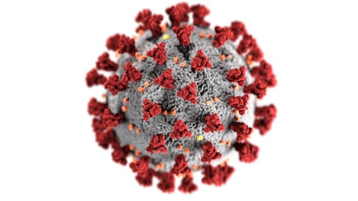
The coronavirus (SARS-CoV-2) is a very large, bristly molecule – with a genome twice as large as that of influenza – studded with spiky flower-like proteins as seen in red in the figure below. It tricks cells in the body into letting it in through a cellular door: a cup-like protein called an ACE2 receptor, which forms part of the nervous system and regulates bodily processes such as blood pressure and inflammation. Latching on to the receptor enables the virus to penetrate the host cell membrane and hijack the cell’s replication machinery, making copies of itself that then wreak havoc throughout the body.

The main function of the body’s immune system is to detect and annihilate invaders such as foreign bacteria and viruses like SARS-CoV-2. First, immune system scouts known as phagocytes – a type of white blood cell – recognize and digest intruder cells. The phagocyte surface then displays a flag or protein fragment of the bacteria or virus, called an antigen, that signals the foreigner’s identity. Other white blood cells called T cells identify the antigen, prompting the immune system arsenal to unleash one of two types of weapon against the assailant.

The two weapons are a different kind of T cell that homes in on infected cells and kills them, and yet another type of white blood cell called a B cell that produces disease fighting antibodies. Antibodies are specialized Y-shaped proteins with a search-and-destroy mission, either inactivating invasive cells directly or tagging them for elimination by phagocytes or other immune system killer cells. Coronavirus vaccines under development include both those that stimulate antibody production, and those that generate copious quantities of T cells.

Most of today’s vaccines utilize the virus itself. This can be in the form of a killed-virus vaccine,  which is produced by growing live virus and then inactivating it chemically, or an attenuated live-virus vaccine, in which live virus is weakened below the level where it can normally cause disease. Both types of vaccine induce the immune system to churn out antibodies.

The measles-mumps-rubella (MMR) vaccine is an example of a weakened virus vaccine; most flu shots are the inactivated type. An inactivated coronavirus vaccine is now in Phase III efficacy testing by Chinese company Sinovac.

Attracting more attention for SARS-CoV-2 are so-called viral vector vaccines. As indicated in the next figure, these are vaccines in which a “guest” virus such as measles (left) or adenovirus (right), which causes upper respiratory infections and related illnesses, is genetically engineered with the gene for the coronavirus spike protein. Key genes in the guest virus are usually disabled so it can’t replicate, but the piggybacking coronavirus gene is unloaded inside the body’s cells, generating antibodies that combat the coronavirus invasion.

CREDIT: SPRINGER NATURE

The only vaccine currently approved for Ebola is a viral vector vaccine manufactured by Johnson & Johnson, who also have a coronavirus vaccine in the works. But the most advanced coronavirus effort is that of the University of Oxford together with AstraZeneca, who have Phase III trials of a viral vector vaccine well underway.           

A third class of defense against the virus using established technologies is protein-based vaccines. Some protein-based vaccines contain fragments of the coronavirus spike protein, or of an important part of it known as the receptor binding domain. The fragments can’t cause disease because they’re not the actual virus, but the immune system is still able to recognize them as coronavirus proteins – triggering production of antibodies. Other protein-based vaccines contain a protein shell that mimics just the outer coat of the coronavirus, so again isn’t infectious but induces antibody production.

Current vaccines for shingles and human papillomavirus (HPV) are in this category. Several companies have Phase I or Phase II trials of a protein-based coronavirus vaccine in progress.

In the next post I’ll review experimental genetic vaccines for the coronavirus, which are based on antibodies, and newer candidates based on a strong T-cell response.

Next: Science on the Attack: The Hunt for a Coronavirus Vaccine (2)

Challenges to the CO2 Global Warming Hypothesis: (3) The Greenhouse Effect Doesn’t Exist

This final post of the present series reviews two papers that challenge the CO₂ global warming hypothesis by purporting to show that there is no greenhouse effect, a heretical claim that even global warming skeptics such as me find hard to accept. According to the authors of the two papers, greenhouses gases in the earth’s atmosphere have played no role in heating the earth, either before or after human emissions of such gases began.

The first paper, published in 2017, utilizes the mathematical tool of dimensional analysis to identify which climatic forcings govern the mean surface temperature of the rocky planets and moons in the solar system that have atmospheres: Venus, Earth, Mars, our Moon, Europa (a moon of Jupiter), Titan (a moon of Saturn) and Triton (a moon of Neptune). A forcing is a disturbance that alters climate, producing heating or cooling.

The paper’s authors, U.S. research scientists Ned Nikolov and Karl Zeller, claim that planetary temperature is controlled by only two forcing variables. These are the total solar irradiance, or total energy from the sun incident on the atmosphere, and the total atmospheric pressure at the planet’s (or moon’s) surface.

In addition to solar irradiance and atmospheric pressure, other forcings considered by Nikolov and Zeller include the near-surface partial pressure and density of greenhouse gases, as well as the mean planetary surface temperature without any greenhouse effect. In their model, the radiative effects integral to the greenhouse effect are replaced by a previously unknown thermodynamic relationship between air temperature, solar heating and atmospheric pressure, analogous to compression heating of the atmosphere. Their findings are illustrated in the figure below, in which T_s is the surface temperature and T_na the temperature with no atmosphere.

A surprising result of their study is that the earth’s natural greenhouse effect – from the greenhouse gases already present in Earth’s preindustrial atmosphere, without any extra CO₂ – warms the planet by a staggering 90 degrees Celsius. This is far in excess of the textbook value of 33 degrees Celsius, or the 18 degrees Celsius calculated by Denis Rancourt and discussed in my previous post. The same 90 degrees Celsius result had also been derived by Nikolov and Zeller from an analytical model, rather than dimensional analysis, in a 2014 paper published under pseudonyms (consisting of their names spelled backwards).

Needless to say, Nikolov and Zeller’s work has been heavily criticized by climate change alarmists and skeptics alike. Skeptical climate scientist Roy Spencer, who has a PhD in meteorology, argues that compression of the atmosphere can’t explain greenhouse heating, because Earth’s average surface temperature is determined not by air pressure, but by the rates at which energy is gained or lost by the surface.

Spencer argues that, if atmospheric pressure causes the lower troposphere (the lowest layer of the atmosphere) to be warmer than the upper troposphere, then the same should be true of the stratosphere, where the pressure at the bottom of the stratosphere is about 100 times larger than that at the top. Yet the bottom of the stratosphere is cooler than the top.

In a reply, Nikolov and Zeller fail to address Spencer’s stratosphere argument, but attempt to defend their work by claiming incorrectly that Spencer ignores the role of adiabatic processes and focuses instead on diabatic radiative processes. Adiabatic processes alter the temperature of a gaseous system without any exchange of heat energy with its surroundings.

The second paper rejecting the greenhouse effect was published in 2009 by German physicists Gerhard Gerlich and Ralf Tscheuschner. They claim that the radiative mechanisms of the greenhouse effect – the absorption of solar shortwave radiation and emission of longwave radiation, which together trap enough of the sun’s heat to make the earth habitable – are fictitious and violate the Second Law of Thermodynamics.

The Second Law forbids the flow of heat energy from a cold region (the atmosphere) to a warmer one (the earth’s surface) without supplying additional energy in the form of external work. However, as other authors point out, the Second Law is not contravened by the greenhouse effect because external energy is provided by downward solar shortwave radiation, which passes through the atmosphere without being absorbed. The greenhouse effect arises from downward emission from the atmosphere of radiation previously emitted upward from the earth.

Furthermore, there’s a net upward transfer of heat energy from the warmer surface to the colder atmosphere when all energy flows are taken into account, including non-radiative convection and latent heat transfer associated with water vapor. Gerlich and Tscheuschner mistakenly insist that heat and energy are separate quantities.

Both of these farfetched claims that the greenhouse effect doesn’t exist therefore stem from misunderstandings about energy.

Next: Science on the Attack: The Hunt for a Coronavirus Vaccine (1)

Challenges to the CO2 Global Warming Hypothesis: (2) Questioning Nature’s Greenhouse Effect

A different challenge to the CO₂ global warming hypothesis from that discussed in my previous post questions the magnitude of the so-called natural greenhouse effect. Like the previous challenge, which was based on a new model for the earth’s carbon cycle, the challenge I’ll review here rejects the claim that human emissions of CO₂ alone have caused the bulk of current global warming.

It does so by disputing the widely accepted notion that the natural greenhouse effect – produced by the greenhouse gases already present in Earth’s preindustrial atmosphere, without any added CO₂ – causes warming of about 33 degrees Celsius (60 degrees Fahrenheit). Without the natural greenhouse effect, the globe would be 33 degrees Celsius cooler than it is now, too chilly for most living organisms to survive.

The controversial assertion about the greenhouse effect was made in a 2011 paper by Denis Rancourt, a former physics professor at the University of Ottawa in Canada, who says that the university opposed his research on the topic. Based on radiation physics constraints, Rancourt finds that the planetary greenhouse effect warms the earth by only 18 degrees, not 33 degrees, Celsius. Since the mean global surface temperature is currently 15.0 degrees Celsius, his result implies a mean surface temperature of -3.0 degrees Celsius in the absence of any atmosphere, as opposed to the conventional value of -18.0 degrees Celsius.

In addition, using a simple two-layer model of the atmosphere, Rancourt finds that the contribution of CO₂ emissions to current global warming is only 0.4 degrees Celsius, compared with the approximately 1 degree Celsius of observed warming since preindustrial times.

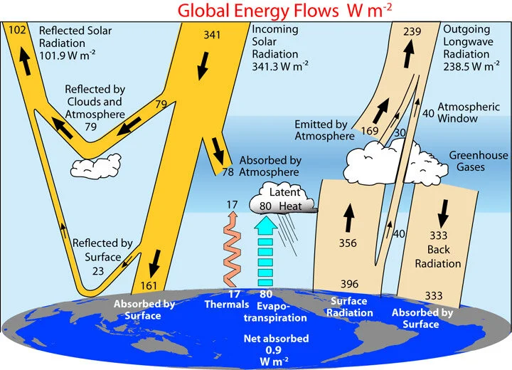
Actual greenhouse warming, he says, is a massive 60 degrees Celsius, but this is tempered by various cooling effects such as evapotranspiration, atmospheric thermals and absorption of incident shortwave solar radiation by the atmosphere. These effects are illustrated in the following figure, showing the earth’s energy flows (in watts per square meter) as calculated from satellite measurements between 2000 and 2004. It should be noted, however, that the details of these energy flow calculations have been questioned by global warming skeptics.

The often-quoted textbook warming of 33 degrees Celsius comes from assuming that the earth’s mean albedo, which measures the reflectivity of incoming sunlight, is the same 0.30 with or without its atmosphere. The albedo with an atmosphere, including the contribution of clouds, can be calculated from the shortwave satellite data on the left side of the figure above, as (79+23)/341 = 0.30. Rancourt calculates the albedo with no atmosphere from the same data, as 23/(23+161) = 0.125, which assumes the albedo is the same as that of the earth’s present surface.

This value is considerably less than the textbook value of 0.30. However, the temperature of an earth with no atmosphere – whether it’s Rancourt’s -4.0 degrees Celsius or a more frigid -19 degrees Celsius – would be low enough for the whole globe to be covered in ice.

Such an ice-encased planet, a glistening white ball as seen from space known as a “Snowball Earth,” is thought to have existed hundreds of millions of years ago. What’s relevant here is that the albedo of a Snowball Earth would be at least 0.4 (the albedo of marine ice) and possibly as high as 0.9 (the albedo of snow-covered ice).

That both values are well above Rancourt’s assumed value of 0.125 seems to cast doubt on his calculation of -4.0 degrees Celsius as the temperature of an earth stripped of its atmosphere. His calculation of CO₂ warming may also be on weak ground because, by his own admission, it ignores factors such as inhomogeneities in the earth’s atmosphere and surface; non-uniform irradiation of the surface; and constraints on the rate of decrease of temperature with altitude in the atmosphere, known as the lapse rate. Despite these limitations, Rancourt finds with his radiation balance approach that his double-layer atmosphere model yields essentially the same result as a single-layer model.

He also concludes that the steady state temperature of Earth’s surface is a sizable two orders of magnitude more sensitive to variations in the sun’s heat and light output, and to variations in planetary albedo due to land use changes, than to increases in the level of CO₂ in the atmosphere. These claims are not accepted even by the vast majority of climate change skeptics, despite Rancourt’s accurate assertion that global warming doesn’t cause weather extremes.

Next: Challenges to the CO2 Global Warming Hypothesis: (3) The Greenhouse Effect Doesn’t Exist

Challenges to the CO2 Global Warming Hypothesis: (1) A New Take on the Carbon Cycle

Central to the dubious belief that humans make a substantial contribution to climate change is the CO₂ global warming hypothesis. The hypothesis is that observed global warming – currently about 1 degree Celsius (1.8 degrees Fahrenheit) since the preindustrial era – has been caused primarily by human emissions of CO₂ and other greenhouse gases into the atmosphere. The CO₂ hypothesis is based on the apparent correlation between rising worldwide temperatures and the CO₂ level in the lower atmosphere, which has gone up by approximately 47% over the same period.

In this series of blog posts, I’ll review several recent research papers that challenge the hypothesis. The first is a 2020 preprint by U.S. physicist and research meteorologist Ed Berry, who has a PhD in atmospheric physics. Berry disputes the claim of the IPCC (Intergovernmental Panel on Climate Change) that human emissions have caused all of the CO₂ increase above its preindustrial level in 1750 of 280 ppm (parts per million), which is one way of expressing the hypothesis.

The IPCC’s CO₂ model maintains that natural emissions of CO₂ since 1750 have remained constant, keeping the level of natural CO₂ in the atmosphere at 280 ppm, even as the world has warmed. But Berry’s alternative model concludes that only 25% of the current increase in atmospheric CO₂ is due to humans and that the other 75% comes from natural sources. Both Berry and the IPCC agree that the preindustrial CO₂ level of 280 ppm had natural origins. If Berry is correct, however, the CO₂ global warming hypothesis must be discarded and another explanation found for global warming.

Natural CO₂ emissions are part of the carbon cycle that accounts for the exchange of carbon between the earth’s land masses, atmosphere and oceans; it includes fauna and flora, as well as soil and sedimentary rocks. Human CO₂ from burning fossil fuels constitutes less than 5% of total CO₂ emissions into the atmosphere, the remaining emissions being natural. Atmospheric CO₂ is absorbed by vegetation during photosynthesis, and by the oceans through precipitation. The oceans also release CO₂ as the temperature climbs.

Berry argues that the IPCC treats human and natural carbon differently, instead of deriving the human carbon cycle from the natural carbon cycle. This, he says, is unphysical and violates the Equivalence Principle of physics. Mother Nature can't tell the difference between fossil fuel CO₂ and natural CO₂. Berry uses physics to create a carbon cycle model that simulates the IPCC’s natural carbon cycle, and then utilizes his model to calculate what the IPCC human carbon cycle should be.

Berry’s physics model computes the flow or exchange of carbon between land, atmosphere, surface ocean and deep ocean reservoirs, based on the hypothesis that outflow of carbon from a particular reservoir is equal to its level or mass in that reservoir divided by its residence time. The following figure shows the distribution of human carbon among the four reservoirs in 2005, when the atmospheric CO₂ level was 393 ppm, as calculated by the IPCC (left panel) and Berry (right panel).

A striking difference can be seen between the two models. The IPCC claims that approximately 61% of all carbon from human emissions remained in the atmosphere in 2005, and no human carbon had flowed to land or surface ocean. In contrast, Berry’s alternative model reveals appreciable amounts of human carbon in all reservoirs that year, but only 16% left in the atmosphere. The IPCC’s numbers result from assuming in its human carbon cycle that human emissions caused all the CO₂ increase above its 1750 level.

The problem is that the sum total of all human CO₂ emitted since 1750 is more than enough to raise the atmospheric level from 280 ppm to its present 411 ppm, if the CO₂ residence time in the atmosphere is as long as the IPCC claims – hundreds of years, much longer than Berry’s 5 to 10 years. The IPCC’s unphysical solution to this dilemma, Berry points out, is to have the excess human carbon absorbed by the deep ocean alone without any carbon remaining at the ocean surface.

Contrary to the IPCC’s claim, Berry says that human emissions don’t continually add CO₂ to the atmosphere, but rather generate a flow of CO₂ through the atmosphere. In his model, the human component of the current 131 (= 411-280) ppm of added atmospheric CO₂ is only 33 ppm, and the other 98 ppm is natural.

The next figure illustrates Berry’s calculations, showing the atmospheric CO₂ level above 280 ppm for the period from 1840 to 2020, including both human and natural contributions. It’s clear that natural emissions, represented by the area between the blue and red solid lines, have not stayed at the same 280 ppm level over time, but have risen as global temperatures have increased. Furthermore, the figure also demonstrates that nature has always dominated the human contribution and that the increase in atmospheric CO₂ is more natural than human.

Other researchers (see, for example, here and here) have come to much the same conclusions as Berry, using different arguments.

Next: Challenges to the CO2 Global Warming Hypothesis: (2) Questioning Nature’s Greenhouse Effect

Science vs Politics: The Precautionary Principle

Greatly intensifying the attack on modern science is invocation of the precautionary principle – a concept developed by 20th-century environmental activists. Targeted at decision making when the available scientific evidence about a potential environmental or health threat is highly uncertain, the precautionary principle has been used to justify a number of environmental policies and laws around the globe. Unfortunately for science, the principle has also been used to support political action on alleged hazards, in cases where there’s little or no evidence for those hazards.

The origins of the precautionary principle can be traced to the application in the early 1970s of the German principle of “Vorsorge” or foresight, based on the belief that environmental damage can be avoided by careful forward planning. The “Vorsorgeprinzip” became the foundation for German environmental law and policies in areas such as acid rain, pollution and global warming. The principle reflects the old adage that “it’s better to be safe than sorry,” and can be regarded as a restatement of the ancient Hippocratic oath in medicine, “First, do no harm.”

Formally, the precautionary principle can be stated as:

When an activity raises threats of harm to human health or the environment, precautionary measures should be taken even if some cause and effect relationships are not fully established scientifically.

But in spite of its noble intentions, the precautionary principle in practice is based far more on political considerations than on science. It’s the “not fully established scientifically” statement that both embraces the principle involved and, at the same time, leaves it open to manipulation and subversion of science.

A notable example of the intrusion of precautionary principle politics into science is the bans on GMO (genetically modified organism) crops by more than half the countries in the European Union. The bans stem from the widespread, fear-based belief that eating genetically altered foods is unsafe, despite the lack of any scientific evidence that GMOs have ever caused harm to a human.

In a 2016 study by the U.S. NAS (National Academy of Sciences, Engineering and Medicine), no substantial evidence was found that the risk to human health was any different for current GMO crops on the market than for their traditionally crossbred counterparts. This conclusion came from epidemiological studies conducted in the U.S. and Canada, where the population has consumed GMO foods since the late 1990s, and similar studies in the UK and Europe, where very few GMO foods are eaten.

The precautionary principle also underlies the UNFCCC (UN Framework Convention on Climate Change), the 1992 treaty that formed the basis for all subsequent political action on global warming. In another post, I’ve discussed the lack of empirical scientific evidence for the narrative of catastrophic anthropogenic (human-caused) climate change. Yet Irrational fear of disastrous consequences of global warming pushes activists to invoke the precautionary principle in order to justify unnecessary, expensive remedies such as those embodied in the Paris Agreement or the Green New Deal.

One of the biggest issues with the precautionary principle is that it essentially advocates risk avoidance. But risk avoidance carries its own risks.

Dangers, great and small, are an accepted part of everyday life. We accept the risk, for example, of being killed or badly injured while traveling on the roads because the risk is outweighed by the convenience of getting to our destination quickly, or by our desire to have fresh food available at the supermarket. Applying the precautionary principle would mean, in addition to the safety measures already in place, reducing all speed limits to 10 mph or less – a clearly impractical solution that would take us back to horse-and-buggy days.  

Another, real-life example of an unintended consequence of the precautionary principle is what happened in Fukushima, Japan in the aftermath of the nuclear accident triggered by a massive earthquake and tsunami in 2011. As described by the authors of a recent discussion paper, Japan’s shutdown of nuclear power production as a safety measure and its replacement by fossil-fueled power raised electricity prices by as much as 38%, decreasing consumption of electricity, especially for heating during cold winters. This had a devastating effect: in the authors’ words,

“Our estimated increase in mortality from higher electricity prices significantly outweighs the mortality from the accident itself, suggesting the decision to cease nuclear production caused more harm than good.”

Adherence to the precautionary principle can also stifle innovation and act as a barrier to technological development. In the worst case, an advantageous technology can be banned because of its potentially negative impact, leaving its positive benefits unrealized. This could well be the case for GMOs. The more than 30 nations that have banned the growing of genetically engineered crops may be shutting themselves off from the promise of producing cheaper and more nutritious food.

The precautionary principle pits science against politics. In an ideal world, the conflict between the two would be resolved wisely. As things are, however, science is often subjugated to the needs and whims of policy makers.

Next: Challenges to the CO₂ Global Warming Hypothesis: (1) A New Take on the Carbon Cycle

Absurd Attempt to Link Climate Change to Cancer Contradicted by Another Medical Study

Extreme weather has already been wrongly blamed on climate change. More outlandish claims have linked climate change to medical and social phenomena such as teenage drinking, declining fertility rates, mental health problems, loss of sleep by the elderly and even Aretha Franklin’s death.

Now the most preposterous claim of all has been made, that climate change causes cancer. A commentary last month in a leading cancer journal contends that climate change is increasing cancer risk through increased exposure to carcinogens after extreme weather events such as hurricanes and wildfires. Furthermore, the article declares, weather extremes impact cancer survival by impeding both patients' access to cancer treatment and the ability of medical facilities to deliver cancer care.

How absurd! To begin with, there’s absolutely no evidence that global warm­ing triggers extreme weather, or even that extreme weather is becoming more frequent. The following figure, depicting the annual number of global hurricanes making landfall since 1970, illustrates the lack of any trend in major hurricanes for the last 50 years – during a period when the globe warmed by ap­proximately 0.6 degrees Celsius (1.1 degrees Fahrenheit). The strongest hurricanes today are no more extreme or devastating than those in the past. If anything, major landfalling hurricanes in the US are tied to La Niña cycles in the Pacific Ocean, not to global warming.

And wildfires in fact show a declining trend over the same period. This can be seen in the next figure, displaying the estimated area worldwide burned by wildfires, by decade from 1900 to 2010. While the number of acres burned annually in the U.S. has gone up over the last 20 years or so, the present burned area is still only a small fraction of what it was back in the 1930s.

Apart from the lack of any connection between climate change and extreme weather, the assertion that hurricanes and wildfires result in increased exposure to carcinogens is dubious. Although hurricanes occasionally cause damage that releases chemicals into the atmosphere, and wildfires generate copious amounts of smoke, these effects are temporary and add very little to the carcinogen load experienced by the average person.

A far greater carcinogen load is experienced continuously by people living in poorer countries who rely on the use of solid fuels, such as coal, wood, charcoal or biomass, for cooking. Incomplete combustion of solid fuels in inefficient stoves results in indoor air pollution that causes respiratory infections in the short term, especially in children, and heart disease or cancer in adults over longer periods of time.

The 2019 Lancet Countdown on Health and Climate Change, an annual assessment of the health effects of climate change, found that mortality from climate-sensitive diseases such as diarrhea and malaria has fallen as the planet has heated, with the exception of dengue fever. Although the Countdown didn’t examine cancer specifically, it did find that the number of people still lacking access to clean cooking fuels and technologies is almost three billion, a number that has fallen by only 1% since 2010.

What this means is that, regardless of ongoing global warming, those billions are still being exposed to indoor carcinogens and are therefore at greater-than-normal risk of later contracting cancer. But the cancer will be despite climate change, not because of it – completely contradicting the claim in the cancer journal that climate change causes cancer.

Because climate change is actually reducing the frequency of hurricanes and wildfires, the commentary’s contention that extreme weather is worsening disruptions to health care access and delivery is also fallacious. Delays due to weather extremes in cancer diagnosis and treatment initiation, and the interruption of cancer care, are becoming less, not more common.

It makes no more sense to link climate change to cancer than to avow that it causes hair loss or was responsible for the creation of the terrorist group ISIS.

Next: Science vs Politics: The Precautionary Principle

How Science Is Being Misused in the Coronavirus Pandemic

Amidst the hysteria over the coronavirus pandemic, politicians constantly assure us that their COVID-19 policy decisions are founded on science. “Following the science” has become the mantra of national and local officials alike.

But the reality is that the various edicts and lockdown measures are based as much on political considerations as science.

One of the hallmarks of science is empirical evidence: true science depends on accumulated observations, not on models or anecdotal data. My previous post discussed the shortcomings of coronavirus models, which rely on assumptions about unknowns such as contagiousness and virus incubation period, and whose only observational data is from past flu epidemics or the current pandemic that the models are attempting to simulate.

Many governments thought they were being informed by science in employing models to forecast the epidemic’s course. But, as leaders discovered in places like Italy and New York where the healthcare system was rapidly overwhelmed, the models were of little use in predicting how many ventilators or how much other equipment they would need. It was their own on-the-spot observations and political experience, not science, that led the way.

Science is not a fountain of wisdom. As a UK sociologist remarks: “Scientists can provide evidence, but acting on that evidence requires political will.” Unfortunately, science can be subverted by the political process, politicians all too often choosing only the evidence that bolsters their existing beliefs. Because politics is more visceral than rational, the evidence and logic intrinsic to science rarely play a big role in political debate.

An example of how politics has trampled science in the coronavirus pandemic is the advice given by the UK government to its citizens on self-isolation (self-quarantine in the U.S.) for those with symptoms of COVID-19.

The UK NHS (National Health Service) says seven days after becoming sick is adequate self-isolation. Yet the WHO (World Health Organization), along with medical experts in many countries, recommends a self-quarantine period of 14 days, based on the observation that the incubation period after exposure to the virus ranges from 1 to 14 days. While scientists can and frequently do disagree, the difference between the NHS and WHO guidelines is purely the result of political interference with science.

Another area where science is being misused is antibody testing.

There’s been much fanfare about the possible use of antibody testing to determine whether someone who has recovered from COVID-19 is immune from reinfection by the virus, and can therefore circulate safely in society. That’s true for many other viruses, but hasn’t yet been established for the coronavirus. And if antibodies do confer protection against reinfection, it’s unknown how long the protection lasts – weeks, months or years.

Compounding these uncertainties is the unreliability of many currently available antibody tests, and the finding that some recovered individuals, as determined by an antibody test, still test positive for the coronavirus – meaning they could still possibly infect others. Recent research suggests these are false positives, arising from harmless fragments of the virus left in the body. However, until there’s evidence to resolve such questions, it’s a mistake for any politician or official to claim that science supports their policy position on antibody testing.

A third example of misuse of science during the pandemic is the debate over prescribing the malaria drug hydroxychloroquine as an early-stage treatment for COVID-19 patients.

It’s not unusual in medicine to prescribe a drug, originally developed to treat a particular illness, as an off-label remedy for another condition. Hydroxychloroquine has for many years been considered a safe and effective treatment for malaria, lupus and rheumatoid arthritis. At the beginning of the coronavirus pandemic, the drug was used successfully to treat COVID-19 in China, France and other countries.

But the use of hydroxychloroquine to treat coronavirus patients in the U.S. has been controversial. President Donald Trump, who took a course of the medication as a preventative measure and touted its potential benefits for sick patients, has been chastised by political opponents for his endorsement of the treatment. Several studies have appeared to show that the drug, not yet officially approved by the FDA (Food and Drug Administration), can cause serious heart problems. One of these studies has, however, been retracted because of doubts over the veracity of the data.

Nevertheless, what’s important about hydroxychloroquine from a scientific viewpoint is that all the studies so far have been epidemiological. As is well known, an epidemiological study can only show a correlation between the drug and certain outcomes, not a clear cause and effect. Epidemiological studies are notoriously misleading, as found in numerous nutritional studies. Delineation of cause and effect requires a clinical trial – a randomized controlled trial, in which the study population is divided randomly into two identical groups, with intervention in only one group and the other group used as a control. So far, no clinical trials of hydroxychloroquine have been completed.

Although science is a powerful tool for understanding the world around us, it has its limitations. It should not be used as an authority in policy making unless the science is firmly grounded in observational evidence.

Next: Absurd Attempt to Link Climate Change to Cancer Contradicted by Another Medical Study

Why Both Coronavirus and Climate Models Get It Wrong

Most coronavirus epidemiological models have been an utter failure in providing advance information on the spread and containment of the insidious virus. Computer climate models are no better, with a dismal track record in predicting the future.

This post compares the similarities and differences of the two types of model. But similarities and differences aside, the models are still just that – models. Although I remarked in an earlier post that epidemiological models are much simpler than climate models, this doesn’t mean they’re any more accurate.     

Both epidemiological and climate models start out, as they should, with what’s known. In the case of the COVID-19 pandemic the knowns include data on the progression of past flu epidemics, and demographics such as population size, age distribution, social contact patterns and school attendance. Among the knowns for climate models are present-day weather conditions, the global distribution of land and ice, atmospheric and ocean currents, and concentrations of greenhouse gases in the atmosphere.

But the major weakness of both types of model is that numerous assumptions must be made to incorporate the many variables that are not known. Coronavirus and climate models have little in common with the models used to design computer chips, or to simulate nuclear explosions as an alternative to actual testing of atomic bombs. In both these instances, the underlying science is understood so thoroughly that speculative assumptions in the models are unnecessary.

Epidemiological and climate models cope with the unknowns by creating simplified pictures of reality involving approximations. Approximations in the models take the form of adjustable numerical parameters, often derisively termed “fudge factors” by scientists and engineers. The famous mathematician John von Neumann once said, “With four [adjustable] parameters I can fit an elephant, and with five I can make him wiggle his trunk.”

One of the most important approximations in coronavirus models is the basic reproduction number R0 (“R naught”), which measures contagiousness. The numerical value of R0 signifies the number of other people that an infected individual can spread the disease to, in the absence of any intervention. As shown in the figure below, R0 for COVID-19 is thought to be in the range from 2 to 3, much higher than for a typical flu at about 1.3, though less than values for other infectious diseases such as measles.

It’s COVID-19’s high R0 that causes the virus to spread so easily, but its precise value is still uncertain. What determines how quickly the virus multiplies, however, is the incubation period, during which an infected individual can’t infect others. Both R0 and the incubation period define the epidemic growth rate. They’re adjustable parameters in coronavirus models, along with factors such as the rate at which susceptible individuals become infectious in the first place, travel patterns and any intervention measures taken.

In climate models, hundreds of adjustable parameters are needed to account for deficiencies in our knowledge of the earth’s climate. Some of the biggest inadequacies are in the representation of clouds and their response to global warming. This is partly because we just don’t know much about the inner workings of clouds, and partly because actual clouds are much smaller than the finest grid scale that even the largest computers can accommodate – so clouds are simulated in the models by average values of size, altitude, number and geographic location. Approximations like these are a major weakness of climate models, especially in the important area of feedbacks from water vapor and clouds.

An even greater weakness in climate models is unknowns that aren’t approximated at all and are simply omitted from simulations because modelers don’t know how to model them. These unknowns include natural variability such as ocean oscillations and indirect solar effects. While climate models do endeavor to simulate various ocean cycles, the models are unable to predict the timing and climatic influence of cycles such as El Niño and La Niña, both of which cause drastic shifts in global climate, or the Pacific Decadal Oscillation. And the models make no attempt whatsoever to include indirect effects of the sun like those involving solar UV radiation or cosmic rays from deep space.

As a result of all these shortcomings, the predictions of coronavirus and climate models are wrong again and again. Climate models are known even by modelers to run hot, by 0.35 degrees Celsius (0.6 degrees Fahrenheit) or more above observed temperatures. Coronavirus models, when fed data from this week, can probably make a reasonably accurate forecast about the course of the pandemic next week – but not a month, two months or a year from now. Dr. Anthony Fauci of the U.S. White House Coronavirus Task Force recently admitted as much.

Computer models have a role to play in science, but we need to remember that most of them depend on a certain amount of guesswork. It’s a mistake, therefore, to base scientific policy decisions on models alone. There’s no substitute for actual, empirical evidence.

Next: How Science Is Being Misused in the Coronavirus Pandemic

Does Planting Trees Slow Global Warming? The Evidence

It’s long been thought that trees, which remove CO₂ from the atmosphere and can live much longer than humans, exert a cooling influence on the planet. But a close look at the evidence reveals that the opposite could be true – that planting more trees may actually have a warming effect.

This is the tentative conclusion reached by a senior scientist at NASA, in evaluating the results of a 2019 study to estimate Earth’s forest restoration potential. It’s the same conclusion that the IPCC (Intergovernmental Panel on Climate Change) came to in a comprehensive 2018 report on climate change and land degradation. Both the 2019 study and IPCC report were based on various forest models.

The IPCC’s findings are summarized in the following figure, which shows how much the global surface temperature is altered by large-scale forestation (crosses) or deforestation (circles) in three different climatic regions: boreal (subarctic), temperate and tropical; the figure also shows how much deforestation affects regional temperatures.

Trees impact the temperature through either biophysical or biogeochemical effects. The principal biophysical effect is changes in albedo, which measures the reflectivity of incoming sunlight. Darker surfaces such as tree leaves have lower albedo and reflect the sun less than lighter surfaces such as snow and ice with higher albedo. Planting more trees lowers albedo, reducing reflection but increasing absorption of solar heat, resulting in global warming.

The second main biophysical effect is changes in evapotranspiration, which is the release of moisture from plant and tree leaves and the surrounding soil. Forestation boosts evapotranspiration, pumping more water vapor into the atmosphere and causing global cooling that competes with the warming effect from reduced albedo.

These competing biophysical effects of forestation are accompanied by a major geochemical effect, namely the removal of CO₂ from the atmosphere by photosynthesis. In photosynthesis, plants and trees take in CO₂ and water, as well as absorbing sunlight, producing energy for growth and releasing oxygen. Lowering the level of the greenhouse gas CO₂ in the atmosphere results in the cooling traditionally associated with planting trees.

The upshot of all these effects, plus other minor contributions, is demonstrated in the figure above. For all three climatic zones, the net global biophysical outcome of large-scale forestation (blue crosses) – primarily from albedo and evapotranspiration changes – is warming.

Additional biophysical data can be inferred from the results for deforestation (small blue circles), simply reversing the sign of the temperature change to show forestation. Doing this indicates global warming again for forestation in boreal and temperate zones, and perhaps slight cooling in the tropics, with regional effects (large blue circles) being more pronounced. There is strong evidence, therefore, from the IPCC report that widespread tree planting results in net global warming from biophysical sources.

The only region for which there is biogeochemical data (red crosses) for forestation – signifying the influence of CO₂ – is the temperate zone, in which forestation results in cooling as expected. Additionally, because deforestation (red dots) results in biogeochemical warming in all three zones, it can be inferred that forestation in all three zones, including the temperate zone, causes cooling.

Which type of process dominates, following tree planting – biophysical or biogeochemical? A careful examination of the figure suggests that biophysical effects prevail in boreal and temperate regions, but biogeochemical effects may have the upper hand in tropical regions. This implies that large-scale planting of trees in boreal and temperate regions will cause further global warming. However, two recent studies (see here and here) of local reforestation have found evidence for a cooling effect in temperate regions.

But even in the tropics, where roughly half of the earth’s forests have been cleared in the past, it’s far from certain that the net result of extensive reforestation will be global cooling. Among other factors that come into play are atmospheric turbulence, rainfall, desertification and the particular type of tree planted.

Apart from these concerns, another issue in restoring lost forests is whether ecosystems in reforested areas will revert to their previous condition and have the same ability as before to sequester CO₂. Says NASA’s Sassan Saatchi, “Once connectivity [to the climate] is lost, it becomes much more difficult for a reforested area to have its species range and diversity, and the same efficiency to absorb atmospheric carbon.”

So, while planting more trees may provide more shade for us humans in a warming world, the environmental benefits are not at all clear.

Next: Why Both Coronavirus and Climate Models Get It Wrong

Coronavirus Epidemiological Models: (3) How Inadequate Testing Limits the Evidence

Hampering the debate over what action to take on the coronavirus, and over which epidemiological model is the most accurate, is a shortage of evidence. Evidence includes the infectiousness of the virus, how readily it’s transmitted, whether infection confers immunity and, if so, for how long. The answers to such questions can only be obtained from individual testing. But testing has been conspicuously inadequate in most countries, being largely limited to those showing symptoms.

We know the number of deaths, those recorded at least, but a big unknown is the total number of people infected. This “evidence fiasco,” as eminent Stanford medical researcher and epidemiologist John Ioannidis describes it, creates great uncertainty about the lethality of COVID-19 and means that reported case fatality rates are meaningless. In Ioannidis’ words, “We don’t know if we are failing to capture infections by a factor of three or 300.”

The following table lists the death rate, expressed as a percentage of known infections, for the countries with the largest number of reported cases as of April 16, and the most recent data for testing rates (per 1,000 people).

As Ioannidis emphasizes, the death rate calculated as a percentage of the number of cases is highly uncertain because of variations in testing rate. And the number of fatalities is likely an undercount, since most countries don’t include those who die at home or in nursing facilities, as opposed to hospitals.

Nevertheless, the data does reveal some stark differences from country to country. Two nations with two of the highest testing rates in the table above – Italy and Germany – show markedly distinct death rates – 13.1% and 2.9%, respectively – despite having not very different numbers of COVID-19 cases. The disparity has been attributed to different demographics and levels of health in Italy and Germany. And two countries with two of the lowest testing rates, France and Turkey, also differ widely in mortality, though Turkey has a lower number of cases to date.

Most countries, including the U.S., lack the ability to test a large number of people and no countries have reliable data on the prevalence of the virus in the population as a whole. Clearly, more testing is needed before we can get a good handle on COVID-19 and be able to make sound policy decisions about the disease.

Two different types of test are necessary. The first is a test to discover how many people are currently infected or not infected, apart from those already diagnosed. A major problem in predicting the spread of the coronavirus has been the existence of asymptomatic individuals, possibly 25% or more of the population, who unknowingly have the disease and transmit the virus to those they come in contact with.

A rapid diagnostic test for infection has recently been developed by U.S. medical device manufacturer Abbott Laboratories. The compact, portable Abbott device, which recently received emergency use authorization from the FDA (U.S. Food and Drug Administration), can deliver a positive (infected) result for COVID-19 in as little as five minutes and a negative (uninfected) result in 13 minutes. Together with a more sophisticated device for use in large laboratories, Abbott expects to provide about 5 million tests in April alone. Public health laboratories using other devices will augment this number by several hundred thousand.

That’s not the whole testing story, however. A negative result in the first test includes both those who have never been infected and those who have been infected but are now recovered. To distinguish between these two groups requires a second test – an antibody test that indicates which members of the community are immune to the virus as a result of previous infection.

A large number of 15-minute rapid antibody tests have been developed around the world. In the U.S., more than 70 companies have sought approval to sell antibody tests in recent weeks, say regulators, although only one so far has received FDA emergency use authorization. It’s not known how reliable the other tests are; some countries have purchased millions of antibody tests only to discover they were inaccurate. And among other unknowns are the level of antibodies it takes to actually become immune and how long antibody protection against the coronavirus actually lasts.       

But there’s no question that both types of test are essential if we’re to accumulate enough evidence to conquer this deadly disease. Empirical evidence is one of the hallmarks of genuine science, and that’s as true of epidemiology as of other disciplines.

Next: Does Planting Trees Slow Global Warming? The Evidence

Coronavirus Epidemiological Models: (2) How Completely Different the Models Can Be

Two of the most crucial predictions of any epidemiological model are how fast the disease in question will spread, and how many people will die from it. For the COVID-19 pandemic, the various models differ dramatically in their projections.

A prominent model, developed by an Imperial College, London research team and described in the previous post, assesses the effect of mitigation and suppression measures on spreading of the pandemic in the UK and U.S. Without any intervention at all, the model predicts that a whopping 500,000 people would die from COVID-19 in the UK and 2.2 million in the more populous U.S. These are the numbers that so alarmed the governments of the two countries.

Initially, the Imperial researchers claimed their numbers could be halved (to 250,000 and 1.1 million deaths, respectively) by implementing a nationwide lockdown of individuals and nonessential businesses. Lead scientist Neil Ferguson later revised the UK estimate drastically downward to 20,000 deaths. But it appears this estimate would require repeating the lockdown periodically for a year or longer, until a vaccine becomes available. Ferguson didn’t give a corresponding reduced estimate for the U.S., but it would be approximately 90,000 deaths if the same scaling applies.

This reduced Imperial estimate for the U.S. is somewhat above the latest projection of a U.S. model, developed by the Institute for Health Metrics and Evaluations at the University of Washington in Seattle. The Washington model estimates the total number of American deaths at about 60,000, assuming national adherence to stringent stay-at-home and social distancing measures. The figure below shows the predicted number of daily deaths as the U.S. epidemic peaks over the coming months, as estimated this week. The peak of 2,212 deaths on April 12 could be as high as 5,115 or as low as 894, the Washington team says.

The Washington model is based on data from local and national governments in areas of the globe where the pandemic is well advanced, whereas the Imperial model primarily relies on data from China and Italy alone.  Peaks in each U.S. state are expected to range from the second week of April through the last week of May.

Meanwhile, a rival University of Oxford team has put forward an entirely different model, which suggests that up to 68% of the UK population may have already been infected. The virus may have been spreading its tentacles, they say, for a month or more before the first death was reported. If so, the UK crisis would be over in two to three months, and the total number of deaths would be below the 250,000 Imperial estimate, due to a high level of herd immunity among the populace. No second wave of infection would occur, unlike the predictions of the Imperial and Washington models.

Nevertheless, that’s not the only possible interpretation of the Oxford results. In a series of tweets, Harvard public health postdoc James Hay has explained that the proportion of the UK population already infected could be anywhere between 0.71% and 56%, according to his calculations using the Oxford model. The higher the percentage infected and therefore immune before the disease began to escalate, the lower the percentage of people still at risk of contracting severe disease, and vice versa.

The Oxford model shares some assumptions with the Imperial and Washington models, but differs slightly in others. For example, it assumes a shorter period during which an infected individual is infectious, and a later date when the first infection occurred. However, as mathematician and infectious disease specialist Jasmina Panovska-Griffiths explains, the two models actually ask different questions. The question asked by the Imperial and Washington groups is: What strategies will flatten the epidemic curve for COVID-19? The Oxford researchers ask the question: Has COVID-19 already spread widely?  

Without the use of any model, Stanford biophysicist and Nobel laureate Michael Levitt has come to essentially the same conclusion as the Oxford team, based simply on an analysis of the available data. Levitt’s analysis focuses on the rate of increase in the daily number of new cases: once this rate slows down, so does the death rate and the end of the outbreak is in sight.

By examining data from 78 of the countries reporting more than 50 new cases of COVID-19 each day, Levitt was able to correctly predict the trajectory of the epidemic in most countries. In China, once the number of newly confirmed infections began to fall, he predicted that the total number of COVID-19 cases would be around 80,000, with about 3,250 deaths – a remarkably accurate forecast, though doubts exist about the reliability of the Chinese numbers. In Italy, where the caseload was still rising, his analysis indicated that the outbreak wasn’t yet under control, as turned out to be tragically true.

Levitt, however, agrees with the need for strong measures to contain the pandemic, as well as earlier detection of the disease through more widespread testing.

Next: Coronavirus Epidemiological Models: (3) How Inadequate Testing Limits the Evidence

Coronavirus Epidemiological Models: (1) What the Models Predict

Amid all the brouhaha over COVID-19 – the biggest respiratory virus threat globally since the 1918 influenza pandemic – confusion reigns over exactly what epidemiological models of the disease are predicting. That’s important as the world begins restricting everyday activities and effectively shutting down national economies, based on model predictions.

In this and subsequent blog posts, I’ll examine some of the models being used to simulate the spread of COVID-19 within a population. As readers will know, I’ve commented at length in this blog on the shortcomings of computer climate models and their failure to accurately predict the magnitude of global warming. 

Epidemiological models, however, are far simpler than climate models and involve far fewer assumptions. The propagation of disease from person to person is much better understood than the vagaries of global climate. A well-designed disease model can help predict the likely course of an epidemic, and can be used to evaluate the most realistic strategies for containing it.

Following the initial coronavirus episode that began in Wuhan, China, various attempts have been made to model the outbreak. One of the most comprehensive studies is a report published last week, by a research team at Imperial College in London, that models the effect of mitigation and suppression control measures on the pandemic spreading in the UK and U.S.

Mitigation focuses on slowing the insidious spread of COVID-19, by taking steps such as requiring home quarantine of infected individuals and their families, and imposing social distancing of the elderly; suppression aims to stop the epidemic in its tracks, by adding more drastic measures such as social distancing of everyone and the closing of nonessential businesses and schools. Both tactics are currently being used not only in the UK and U.S., but also in many other countries – especially in Italy, hit hard by the epidemic.

The model results for the UK are illustrated in the figure below, which shows how the different strategies are expected to affect demand for critical care beds in UK hospitals over the next few months. You can see the much-cited “flattening of the curve,” referring to the bell-shaped curve that portrays the peaking of critical care cases, and related deaths, as the disease progresses. The Imperial College model assumes that 50% of those in critical care will die, based on expert clinical opinion. In the U.S., the epidemic is predicted to be more widespread than in the UK and to peak slightly later.

What set alarm bells ringing was the model’s conclusion that, without any intervention at all, approximately 0.5 million people would die from COVID-19 in the UK and 2.2 million in the more populous U.S. But these numbers could be halved (to 250,000 and 1.1-1.2 million deaths, respectively) if all the proposed mitigation and suppression measures are put into effect, say the researchers.

Nevertheless, the question then arises of how long such interventions can or should be maintained. The blue shading in the figure above shows the 3-month period during which the interventions are assumed to be enforced. But because there is no cure for the disease at present, it’s possible that a second wave of infection will occur once interventions are lifted. This is depicted in the next figure, assuming a somewhat longer 5-month period of initial intervention.

The advantage of such a delayed peaking of the disease’s impact would be a lessening of pressure on an overloaded healthcare system, allowing more time to build up necessary supplies of equipment and reducing critical care demand – in turn reducing overall mortality. In addition, stretching out the timeline for a sufficiently long time could help bolster herd immunity. Herd immunity from an infectious disease results when enough people become immune to the disease through either recovery or vaccination, both of which reduce disease transmission. A vaccine, however, probably won’t be available until 2021, even with the currently accelerated pace of development.

Whether the assumptions behind the Imperial College model are accurate is an issue we’ll look at in a later post. The model is highly granular, reaching down to the level of the individual and based on high-resolution population data, including census data, data from school districts, and data on the distribution of workplace size and commuting distance. Contacts between people are examined within a household, at school, at work and in social settings.

The dilemma posed by the model’s predictions is obvious. It’s necessary to balance minimizing the death rate from COVID-19 with the social and economic disruption caused by the various interventions, and with the likely period over which the interventions can be maintained.

Next: Coronavirus Epidemiological Models: (2) How Completely Different the Models Can Be

Science on the Attack: Cancer Immunotherapy

As a diversion from my regular blog posts examining how science is under attack, occasional posts such as this one will showcase examples of science nevertheless on the attack – to illustrate the power of the scientific method in tackling knotty problems, even when the discipline itself is under siege. This will exclude technology, which has always thrived. The first example is from the field of medicine: cancer immunotherapy.

Cancer is a vexing disease, in fact a slew of different diseases, in which abnormal cells proliferate uncontrollably and can spread to healthy organs and tissues. It’s one of the leading causes of death worldwide, especially in high-income countries. Each type of cancer, such as breast, lung or prostate, has as many as 10 different sub-types, vastly complicating efforts to conquer the disease.

Although the role of the body’s immune system is to detect and destroy abnormal cells, as well as invaders like foreign bacteria and viruses, cancer can evade the immune system through several mechanisms that shut down the immune response.

One mechanism involves the immune system deploying T-cells – a type of white blood cell – to recognize abnormal cells. It does this by looking for flags or protein fragments called antigens displayed on the cell surface that signal the cell’s identity. The T-cells, sometimes called the warriors of the immune system, identify and then kill the offending cells.

But the problem is that cancer cells can avoid annihilation by deactivating a switch on the T-cell known as an immune checkpoint, the purpose of which is to prevent T-cells from becoming over zealous and generating too powerful an immune response. Switching off the checkpoint altogether takes the T-cell out of the action and allows the cancer to grow. The breakthrough of cancer immunotherapy was in discovering drugs that can act as checkpoint inhibitors, which keep the checkpoint activated or switched on at all times and therefore enable the immune system to do its job in attacking the cancerous cells.

However, such a discovery wasn’t an easy task. Attempts to harness the immune system to fight cancer go back over 100 years, but none of these attempts worked successfully on a consistent basis. The only options available to cancer patients were from the standard regimen of surgery, chemotherapy, radiation and hormonal treatments.

In what the British Society for Immunology described as “one of the most extraordinary breakthroughs in modern medicine,” researchers James P. Allison and Tasuku Honjo were awarded the 2018 Nobel Prize in Physiology or Medicine for their discoveries of different checkpoint inhibitor drugs – discoveries that represented the culmination of over a decade’s painstaking laboratory work. Allison explored one type of checkpoint inhibitor (known as CTLA-4), Honjo another one (known as PD-1).

Early clinical tests of both types of inhibitor showed spectacular results. In several patients with advanced melanoma, an aggressive type of skin cancer, the cancer completely disappeared when treated with a drug based on Allison’s research. In patients with other types of cancer such as lung cancer, renal cancer and lymphoma, treatment with a drug based on Honjo’s research resulted in long-term remission, and may have even cured metastatic cancer – previously not considered treatable.

Yet despite this initial promise, it’s been found that checkpoint inhibitor immunotherapy is effective for only a small portion of cancer patients: genetic differences are no doubt at play. States Dr. Roy Herbst, chief of medical oncology at Yale Medicine, “The sad truth about immunotherapy treatment in lung cancer is that it shrinks tumors in only about one or two out of 10 patients.” More research and possibly drug combinations will be needed, Dr. Herbst says, to extend the revolutionary new treatment to more patients.

Another downside is possible side effects from immune checkpoint drugs, caused by overstimulation of the immune system and consequent autoimmune reactions in which the immune system attacks normal, healthy tissue. But such reactions are usually manageable and not life-threatening.

Cancer immunotherapy is but one of many striking recent advances in the medical field, illustrating how the biomedical sciences can be on the attack even as they come under assault, especially from medical malfeasance in the form of irreproducibility and fraud.

Next: Coronavirus Epidemiological Models: (1) What the Models Predict

The Futility of Action to Combat Climate Change: (2) Political Reality

In the previous post, I showed how scientific and engineering realities make the goal of taking action to combat climate change inordinately expensive and unattainable in practice for decades to come, even if climate alarmists are right about the need for such action. This post deals with the equally formidable political realities involved.

By far the biggest barrier is the unlikelihood that the signatories to the 2015 Paris Agreement will have the political will to adhere to their voluntary pledges for reducing greenhouse gas emissions. Lacking any enforcement mechanism, the agreement is merely a “feel good” document that allows nations to signal virtuous intentions without actually having to make the hard decisions called for by the agreement. This reality is tacitly admitted by all the major CO₂ emitters.

Evidence that the Paris Agreement will achieve little is contained in the figure below, which depicts the ability of 58 of the largest emitters, accounting for 80% of the world’s greenhouse emissions, to meet the present goals of the accord. The goals are to hold “the increase in the global average temperature to well below 2 degrees Celsius (3.6 degrees Fahrenheit) above pre-industrial levels,” preferably limiting the increase to only 1.5 degrees Celsius (2.7 degrees Fahrenheit).

It’s seen that only seven nations have declared emission reductions big enough to reach the Paris Agreement’s goals, including just one of the largest emitters, India. The seven largest emitters, apart from India which currently emits 7% of the world’s CO₂, are China (28%), the USA (14%), Russia (5%), Japan (3%), Germany (2%, biggest in the EU) and South Korea (2%). The EU designation here includes the UK and 27 European nations.

As the following figure shows, annual CO₂ emissions from both China and India are rising, along with those from the other developing nations (“Rest of world”). Emissions from the USA and EU, on the other hand, have been steady or falling for several decades. Ironically, the USA’s emissions in 2019, which dropped by 2.9% from the year before, were no higher than in 1993 – despite the country’s withdrawal from the Paris Agreement.

As the developing nations, including China and India, currently account for 76% of global emissions, it’s difficult to imagine that the world as a whole will curtail its emissions anytime soon.

China, although a Paris Agreement signatory, has declared its intention of increasing its annual CO₂ emissions until 2030 in order to fully industrialize – a task requiring vast amounts of additional energy, mostly from fossil fuels. The country already has over 1,000 GW of coal-fired power capacity and another 120 GW under construction. China is also financing or building 250 GW of coal-fired capacity as part of its Belt and Road Initiative across the globe. Electricity generation in China from burning coal and natural gas accounted for 70% of the generation total in 2018, compared with 26% from renewables, two thirds of which came from hydropower.

India, which has also ratified the Paris Agreement, believes it can meet the agreement’s aims even while continuing to pour CO₂ into the atmosphere. Coal’s share of Indian primary energy consumption, which is predominantly for electricity generation and steelmaking, is expected to decrease slightly from 56% in 2017 to 48% in 2040. However, achieving even this reduction depends on doubling the share of renewables in electricity production, an objective that may not be possible because of land acquisition and funding barriers.

Nonetheless, it’s not China nor India that stand in the way of making the Paris Agreement a reality, but rather the many third world countries who want to reach the same standard of living as the West – a lifestyle that has been attained through the availability of cheap, fossil fuel energy. In Africa today, for example, 600 million people don’t have access to electricity and 900 million are forced to cook with primitive stoves fueled by wood, charcoal or dung, all of which create health and environmental problems. Coal-fired electricity is the most affordable remedy for the continent.

In the words of another writer, no developing country will hold back from increasing their CO₂ emissions “until they have achieved the same levels of per capita energy consumption that we have here in the U.S. and in Europe.” This drive for a better standard of living, together with the lack of any desire on the part of industrialized countries to lower their energy consumption, spells disaster for realizing the lofty goals of the Paris Agreement.

Next: Science on the Attack: Cancer Immunotherapy

The Futility of Action to Combat Climate Change: (1) Scientific and Engineering Reality

Amidst the clamor for urgent action to supposedly combat climate change, the scientific and engineering realities of such action are usually overlooked. Let’s imagine for a moment that we humans are indeed to blame for global warming and that catastrophe is imminent without drastic measures to curb fossil fuel emissions – views not shared by climate skeptics like myself.

In this and the subsequent blog post, I’ll show how proposed mitigation measures are either impractical or futile. We’ll start with the 2015 Paris Agreement – the international agreement on cutting greenhouse gas emissions, which 195 nations, together with many of the world’s scientific societies and national academies, have signed on to.

The agreement endorses the assertion that global warming comes largely from our emissions of greenhouse gases, and commits its signatories to “holding the increase in the global average temperature to well below 2 degrees Celsius (3.6 degrees Fahrenheit) above pre-industrial levels,” preferably limiting the increase to only 1.5 degrees Celsius (2.7 degrees Fahrenheit). According to NASA, current warming is close to 1 degree Celsius (1.8 degrees Fahrenheit).

How realistic are these goals? To achieve them, the Paris Agreement requires nations to declare a voluntary “nationally determined contribution” toward emissions reduction. However, it has been estimated by researchers at MIT (Massachusetts Institute of Technology) that, even if all countries were to follow through with their voluntary contributions, the actual mitigation of global warming by 2100 would be at most only about 0.2 degrees Celsius (0.4 degrees Fahrenheit).

Higher estimates, ranging up to 0.6 degrees Celsius (1.1 degrees Fahrenheit), assume that countries boost their initial voluntary emissions targets in the future. The agreement actually stipulates that countries should submit increasingly ambitious targets every five years, to help attain its long-term temperature goals. But the targets are still voluntary, with no enforcement mechanism.

Given that most countries are already falling behind their initial pledges, mitigation of more than 0.2 degrees Celsius (0.4 degrees Fahrenheit) by 2100 seems highly unlikely. Is it worth squandering the trillions of dollars necessary to achieve such a meager gain, even if the notion that we can control the earth’s thermostat is true?     

Another reality check is the limitations of renewable energy sources, which will be essential to our future if the world is to wean itself off fossil fuels that today supply almost 80% of our energy needs. The primary renewable technologies are wind and solar photovoltaics. But despite all the hype, wind and solar are not yet cost competitive with cheaper coal, oil and gas in most countries, when subsidies are ignored. Higher energy costs can strangle a country’s economy.

Source: BP

And it will be many years before renewables are practical alternatives to fossil fuels. It’s generally unappreciated by renewable energy advocates that full implementation of a new technology can take many decades. That’s been demonstrated again and again over the past century in areas as diverse as electronics and steelmaking.

The claim is often made, especially by proponents of the so-called Green New Deal, that scale-up of wind and solar power could be accomplished quickly by mounting an effort comparable to the U.S. moon landing program in the 1960s. But the claim ignores the already mature state of several technologies crucial to that program at the outset. Rocket technology, for example, had been developed by the Germans and used to terrify Londoners in the UK during World War II. The vacuum technology needed for the Apollo crew modules and spacesuits dates from the beginning of the 20th century.

Such advantages don’t apply to renewable energy. The main engineering requirements for widespread utilization of wind and solar power are battery storage capability, to store energy for those times when the wind stops blowing or the sun isn’t shining, and redesign of the electric grid.

But even in the technologically advanced U.S., battery storage is an order of magnitude too expensive today for renewable electricity to be cost competitive with electricity generated from fossil fuels. That puts battery technology where rocket technology was more than 25 years before Project Apollo was able to exploit its use in space. Likewise, conversion of the U.S. power grid to renewable energy would cost trillions of dollars – and, while thought to be attainable, is currently seen as merely “aspirational.”

The bottom line for those who believe we must act urgently on the climate “emergency”: it’s going to take a lot of time and money to do anything at all, and whatever we do may make little difference to the global climate anyway.

Next: The Futility of Action to Combat Climate Change: (2) Political Reality