Antarctica Sending Mixed Climate Messages

Antarctica, the earth’s coldest and least-populated continent, is an enigma when it comes to global warming.

While the huge Antarctic ice sheet is known to be shedding ice around its edges, it may be growing in East Antarctica. Antarctic sea ice, after expanding slightly for at least 37 years, took a tumble in 2017 and reached a record low in 2023. And recent Antarctic temperatures have swung from record highs to record lows. No one is sure what’s going on.

The influence of global warming on Antarctica’s temperatures is uncertain. A 2021 study concluded that both East Antarctica and West Antarctica have cooled since the beginning of the satellite era in 1979, at rates of 0.70 degrees Celsius (1.3 degrees Fahrenheit) per decade and 0.42 degrees Celsius (0.76 degrees Fahrenheit) per decade, respectively. But over the same period, the Antarctic Peninsula (on the left in the adjacent figure) has warmed at a rate of 0.18 degrees Celsius (0.32 degrees Fahrenheit) per decade.

During the southern summer, two locations in East Antarctica recorded record low temperatures early this year. At the Concordia weather station, located at the 4 o’clock position from the South Pole, the mercury dropped to -51.2 degrees Celsius (-60.2 degrees Fahrenheit) on January 31, 2023. This marked the lowest January temperature recorded anywhere in Antarctica since the first meteorological observations there in 1956.

Two days earlier on January 29, 2023, the nearby Vostok station, about 400 km (250) miles closer to the South Pole, registered a low temperature of -48.7 degrees Celsius (-55.7 degrees Fahrenheit), that location’s lowest January temperature since 1957. Vostok has the distinction of reporting the lowest temperature ever recorded in Antarctica, and also the world record low, of -89.2 degrees Celsius (-128.6 degrees Fahrenheit) on July 21, 1984.

Barely a year before, however, East Antarctica had experienced a heat wave, when the temperature soared to -10.1 degrees Celsius (13.8 degrees Fahrenheit) at the Concordia station on March 18, 2022. This balmy reading was the highest recorded hourly temperature at that weather station since its establishment in 1996, and 20 degrees Celsius (36 degrees Fahrenheit) above the previous March record high there. Remarkably, the temperature remained above the previous March record for three consecutive days, including nighttime.

Antarctic sea ice largely disappears during the southern summer and reaches its maximum extent in September, at the end of winter. The two figures below illustrate the winter maximum extent in 2023 (left) and the monthly variation of Antarctic sea ice extent this year from its March minimum to the September maximum (right).

The black curve on the right depicts the median extent from 1981 to 2010, while the dashed red and blue curves represent 2022 and 2023, respectively. It's clear that Antarctic sea ice in 2023 has lagged the median and even 2022 by a wide margin throughout the year. The decline in summer sea ice extent has now persisted for six years, as seen in the following figure which shows the average monthly extent since satellite measurements began, as an anomaly from the median value.

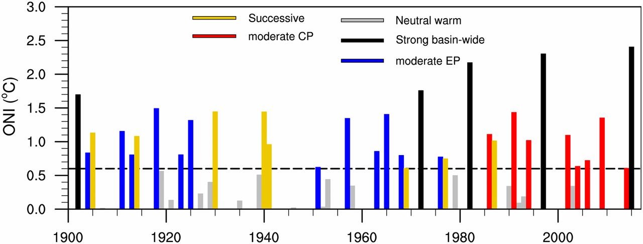
The overall trend from 1979 to 2023 is an insignificant 0.1% per decade relative to the 1981 to 2010 median. Yet a prolonged  increase above the median occurred from 2008 to 2017, followed by the six-year decline since then. The current downward trend has sparked much debate and several possible reasons have been put forward, not all of which are linked to global warming. One analysis attributes the big losses of sea ice in 2017 and 2023 to extra strong El Niños.

Melting of the Antarctic ice sheet is currently causing sea levels to rise by 0.4 mm (16 thousandths of an inch) per year, contributing about 10% of the global total. But the ice loss is not uniform across the continent, as seen in the next figure showing changes in Antarctic ice sheet mass since 2002.

In the image on the right, light blue shades indicate ice gain while orange and red shades indicate ice loss. White denotes areas where there has been very little or no change in ice mass since 2002; gray areas are floating ice shelves whose mass change is not measured by this satellite method.

You can see that East Antarctica has experienced modest amounts of ice gain, which is due to warming-enhanced snowfall. Nevertheless, this gain has been offset by significant loss of ice in West Antarctica over the same period, largely from melting of glaciers – which is partly caused by active volcanoes underneath the continent. While the ice sheet mass declined at a fairly constant rate of 133 gigatonnes (147 gigatons) per year from 2002 to 2020, it appears that the total mass may have reached a minimum and is now on the rise again.

Despite the hullabaloo about its melting ice sheet and shrinking sea ice, what happens next in Antarctica continues to be a scientific mystery.

Next: Two Statistical Studies Attempt to Cast Doubt on the CO2 Narrative

No Evidence That Today’s El Niños Are Any Stronger than in the Past

The current exceptionally strong El Niño has revived discussion of a question which comes up whenever the phenomenon recurs every two to seven years: are stronger El Niños caused by global warming? While recent El Niño events suggest that in fact they are, a look at the historical record shows that even stronger El Niños occurred in the distant past.

El Niño is the warm phase of ENSO (the El Niño – Southern Oscillation), a natural ocean cycle that causes drastic temperature fluctuations and other climatic effects in tropical regions of the Pacific. Its effect on atmospheric temperatures is illustrated in the figure below. Warm spikes such as those in 1997-98, 2009-10, 2014-16 and 2023 are due to El Niño; cool spikes like those in 1999-2001 and 2008-09 are due to the cooler La Niña phase.

A slightly different temperature record, of selected sea surface temperatures in the El Niño region of the Pacific, averaged yearly from 1901 to 2017, is shown in the next figure from a 2019 study.

Here the baseline is the mean sea surface temperature over the 1901-2017 interval, and the black dashed line at 0.6 degrees Celsius is defined by the study authors as the threshhold for an El Niño event. The different colors represent various regional types of El Niño; the gray bars mark warm years in which no El Niño developed.

This year’s gigantic spike in the tropospheric temperature to 0.93 degrees Celsius (1.6 degrees Fahrenheit) – a level that set alarm bells ringing – is clearly the strongest El Niño by far in the satellite record. Comparison of the above two figures shows that it is also the strongest since 1901. So it does indeed appear that El Niños are becoming stronger as the globe warms, especially since 1960.

Nevertheless, such a conclusion is ill-considered as there is evidence from an earlier study that strong El Niños have been plentiful in the earth’s past.

As I described in a previous post, a team of German paleontologists established a complete record of El Niño events going back 20,000 years, by examining marine sediment cores drilled off the coast of Peru. The cores contain an El Niño signature in the form of tiny, fine-grained stone fragments, washed into the sea by multiple Peruvian rivers following floods in the country caused by heavy El Niño rainfall.

The research team classified the flood signal as very strong when the concentration of stone fragments, known as lithics, was more than two standard deviations above the centennial mean. The frequency of these very strong events over the last 12,000 years is illustrated in the next figure; the black and gray bars show the frequency as the number of 500- and 1,000-year floods, respectively. Radiocarbon dating of the sediment cores was used to establish the timeline.

A more detailed record is presented in the following figure, showing the variation over 20,000 years of the sea surface temperature off Peru (top), the lithic concentration (bottom) and a proxy for lithic concentration (center). Sea surface temperatures were derived from chemical analysis of the marine sediment cores.

You can see that the lithic concentration and therefore El Niño strength were high around 2,000 and 10,000 years ago – approximately the same periods when the most devastating floods occurred. The figure also reveals the absence of strong El Niño activity from 5,500 to 7,500 years ago, a dry interval without any major Peruvian floods as reflected in the previous figure.

If you examine the lithic plots carefully, you can also see that the many strong El Niños approximately 2,000 and 10,000 years ago were several times stronger (note the logarithmic concentration scale) than current El Niños on the far left of the figure. Those two periods were warmer than today as well, being the Roman Warm Period and the Holocene Thermal Maximum, respectively.

So there is nothing remarkable about recent strong El Niños.

Despite this, the climate science community is still uncertain about the global warming question. The 2019 study described above found that since the 1970s, formation of El Niños has shifted from the eastern to the western Pacific, where ocean temperatures are higher. From this observation, the study authors concluded that future El Niños may intensify. However, they qualified their conclusion by stating that:

… the root causes of the observed background changes in the later part of the 20th century remain elusive … Natural variability may have added significant contributions to the recent warming.

Recently, an international team of 17 scientists has conducted a theoretical study of El Niños since 1901 using 43 climate models, most of which showed the same increase in El Niño strength since 1960 as the actual observations. But again, the researchers were unable to link this increase to global warming, declaring that:

Whether such changes are linked to anthropogenic warming, however, is largely unknown.

The researchers say that resolution of the question requires improved climate models and a better understanding of El Niño itself. Some climate models show El Niño becoming weaker in the future.

Next: Antarctica Sending Mixed Climate Messages

Targeting Farmers for Livestock Greenhouse Gas Emissions Is Misguided

Farmers in many countries are increasingly coming under attack over their livestock herds. Ireland’s government is contemplating culling the country’s cattle herds by 200,000 cows to cut back on methane (CH₄) emissions; the Dutch government plans to buy out livestock farmers to lower emissions of CH₄ and nitrous oxide (N₂O) from cow manure; and New Zealand is close to taxing CH₄ from cow burps.

But all these measures, and those proposed in other countries, are misguided and shortsighted – for multiple reasons.

The thrust behind the intended clampdown on the farming community is the estimated 11-17% of current greenhouse gas emissions from agriculture worldwide, which contribute to global warming. Agricultural CH₄, mainly from ruminant animals, accounted for approximately 4% of total greenhouse gas emissions in the U.S. in 2021, according to the EPA (Environmental Protection Agency), while N₂O accounted for another 5%.

The actual warming produced by these two greenhouse gases depends on their so-called “global warming potential,” a quantity determined by three factors: how efficiently the gas absorbs heat, its lifetime in the atmosphere, and its atmospheric concentration. The following table illustrates these factors for CO₂, CH₄ and N₂O, together with their comparative warming effects.

The conventional global warming potential (GWP) is a dimensionless metric, in which the GWP per molecule of a particular greenhouse gas is normalized to that of CO₂; the GWP takes into account the atmospheric lifetime of the gas. The table shows both GWP-20 and GWP-100, the warming potentials calculated over a 20-year and 100-year time horizon, respectively.

The final column shows what I call weighted GWP values, as percentages of the CO₂ value, calculated by multiplying the conventional GWP by the ratio of the rate of concentration increase for that gas to that of CO₂. The weighted GWP indicates how much warming CH₄ or N₂O causes relative to CO₂.

Over a 100-year time span, you can see that both CH₄ and N₂O exert essentially the same warming influence, at 10% of CO₂ warming. But over a 20-year interval, CH₄ has a stronger warming effect than N₂O, at 27% of CO₂ warming, because of its shorter atmospheric lifetime which boosts the conventional GWP value from 30 (over 100 years) to 83.

However, the actual global temperature increase from CH₄ and N₂O – concern over which is the basis for legislation targeting the world’s farmers – is small. Over a 20-year period, the combined contribution of these two gases is approximately 0.075 degrees Celsius (0.14 degrees Fahrenheit), assuming that all current warming comes from CO₂, CH₄ and N₂O combined, and using a value of 0.14 degrees Celsius (0.25 degrees Fahrenheit) per decade for the current warming rate.

But, as I’ve stated in many previous posts, at least some current warming is likely to be from natural sources, not greenhouse gases. So the estimated 20-year temperature rise of 0.075 degrees Celsius (0.14 degrees Fahrenheit) is probably an overestimate. The corresponding number over 100 years, also an overestimate, is 0.23 degrees Celsius (0.41 degrees Fahrenheit).

Do such small, or even smaller, gains in temperature justify the shutting down of agriculture? Farmers around the globe certainly don’t think so, and for good reason.

First, CH₄ from ruminant animals such as cows, sheep and goats accounts for only 4% of U.S. greenhouse emissions as noted above, compared with 29% from transportation, for example. And our giving up eating meat and dairy products would have little impact on global temperatures. Removing all livestock and poultry from the U.S. food system would only reduce global greenhouse gas emissions by 0.36%, a study has found.

Other studies have shown that the elimination of all livestock from U.S. farms would leave our diets deficient in vital nutrients, including high-quality protein, iron and vitamin B12 that meat provides, says the Iowa Farm Bureau.

Furthermore, as agricultural advocate Kacy Atkinson argues, the methane that cattle burp out during rumination breaks down in 10 to 15 years into CO₂ and water. The grasses that cattle graze on absorb that CO₂, and the carbon gets sequestered in the soil through the grasses’ roots.

Apart from cow manure management, the largest source of N₂O emissions worldwide is the application of nitrogenous fertilizers to boost crop production. Greatly increased use of nitrogen fertilizers is the main reason for massive increases in crop yields since 1961, part of the so-called green revolution in agriculture.

The figure below shows U.S. crop yields relative to yields in 1866 for corn, wheat, barley, grass hay, oats and rye. The blue dashed curve is the annual agricultural usage of nitrogen fertilizer in megatonnes (Tg). The strong correlation with crop yields is obvious.

Restricting fertilizer use would severely impact the world’s food supply. Sri Lanka’s ill-conceived 2022 ban of nitrogenous fertilizer (and pesticide) imports caused a 30% drop in rice production, resulting in widespread hunger and economic turmoil – a cautionary tale for any efforts to extend N₂O reduction measures from livestock to crops.

Next: No Evidence That Today’s El Niños Are Any Stronger than in the Past

Estimates of Economic Losses from El Niños Are Far-fetched

A recent study makes the provocative claim that some of the most intense past El Niño events cost the global economy from $4 trillion to $6 trillion over the following years. That’s two orders of magnitude higher than previous estimates, but almost certainly wrong.

One reason for the enormous difference is that earlier estimates only examined the immediate economic toll, whereas the new study estimated cumulative losses over the five-year period after a warming El Niño. The study authors say, correctly, that the economic downturn triggered by this naturally occurring climate cycle can last that long.

However, even when this drawn-out effect is taken into account, the new study’s cost estimates are still one order of magnitude greater than other estimates in the scientific literature, such as those of the University of Colorado’s Roger Pielke Jr., who studies natural disasters. His estimated time series of total weather disaster losses as a proportion of global GDP from 1990 to 2020 is shown in the figure below.

The accounting used in the new study includes the “spatiotemporal heterogeneity of El Niño teleconnections,” teleconnections being links between weather phenomena at widely separated locations. Country-level teleconnections are based on correlations between temperature or rainfall in that country, and indexes commonly used to define El Niño and its cooling counterpart, La Niña. Teleconnections are strongest in the tropics and weaker in midlatitudes.

The researchers’ accounting procedure estimates total losses from the 1997-98 El Niño at a staggering $5.7 trillion by 2003, compared with a previous estimate of only $36 billion in the immediate aftermath of the event. For the earlier 1982-83 El Niño, the study estimates the total costs at $4.1 trillion by 1988. The calculated global distribution of GDP losses following both events is illustrated in the next figure.

To see how implausible these trillion-dollar estimates are, it’s only necessary to refer to Pielke’s graph above, which relies on official data from the insurance industry (including leading reinsurance company Munich Re) and the World Bank. His graph indicates that the peak loss from all 1998 weather disasters was 0.38% of global GDP for that year.

As El Niño was not the only disaster in 1998 – others include floods and hurricanes – this number represents an upper limit for instant El Niño losses. Using a value for global GDP in 1998 of $31,533 billion in current U.S. dollars, 0.38% was a maximum instant loss of $120 billion. Over a subsequent 5-year period, the maximum loss would have been 5 times as much, or $600 billion assuming the same annual loss each year which is undoubtedly an overestimate.

This inflated estimate of $600 billion is still an order of magnitude smaller than the study’s $5.7 trillion by 2003. In reality, the discrepancy is larger yet because the actual 5-year loss was likely much less than $600 billion as just discussed.

Two other observations about Pielke’s graph cast further doubt on the methodology of the researchers’ accounting procedure. First, the strongest El Niños in that 21-year period were those in 1997-98, 2009-10 and 2014-16. The graph does indeed show peaks in 1998-99 and in 2017, one year after a substantial El Niño – but not in 2011 following the 2009-10 event. This alone suggests that financial losses from El Niño are not as large as the researchers think.

Furthermore, there’s a strong peak in 2005, the largest in the 21 years of the graph, which doesn’t correspond to any substantial El Niño. The implication is that losses from other types of weather disaster can dominate losses from El Niño.

It’s important to get an accurate handle on economic losses from El Niño and other weather disasters, in case global warming exacerbates such events in the future – although, as I’ve written extensively, there’s no evidence to date that this is happening yet. Effects of El Niño include catastrophic flooding in the western Americas, flooding or episodic droughts in Australia, and coral bleaching.

The study authors stand by their research, however, estimating that the 2023 El Niño could hold back the global economy by $3 trillion over the next five years, a figure not included in their paper. But others are more skeptical. Climate economist Gary Yohe commented that “the enormous estimates cannot be explained simply by forward-looking accounting.” And Mike McPhaden, a senior scientist at NOAA (the U.S. National Oceanic and Atmospheric Administration) who was not involved in the research, called the study “provocative.”

Next: Targeting Farmers for Livestock Greenhouse Gas Emissions Is Misguided

Challenges to the CO2 Global Warming Hypothesis: (9) Rotation of the Earth’s Core as the Source of Global Warming

Yet another challenge to the CO₂ global warming hypothesis, but one radically different from all the other challenges I’ve discussed in this series, hypothesizes that global warming or cooling result entirely from the slight speeding up or slowing down of the earth’s rotating inner core.

Linking the earth’s rotation to its surface temperature is not a new idea and has been discussed by several geophysicists over the last 50 years. What is new is the recent (2023) discovery that changes in global temperature follow changes in the earth’s rotation rate that in turn follow changes in the rotation rate of the inner core, both with a time delay. This discovery underlies the postulate that the earth’s temperature is regulated by rotational variations of the inner core, not by CO₂.

The history and recent developments of the rotational hypothesis have been summarized in a recent paper by Australian Richard Mackey. The apparently simplistic hypothesis, which is certain to raise scientific eyebrows, does, however, meet the requirements for its scientific validation or rejection: it makes a prediction that can be tested against observation.

As Mackey explains, the prediction is that our current bout of global warming will come to an end in 2025, when global cooling will begin.

The prediction is based on the geophysical findings that shifts in the earth’s temperature appear to occur about eight years after the planet’s rotation rate changes, and the earth’s rotation rate changes eight years after the inner core’s rotation rate does. Because the inner core’s rotation rate began to slow around 2009, cooling should set in around 16 years later in 2025, according to the rotational hypothesis.

As illustrated in the figure below, the partly solid inner core is surrounded by the liquid metal outer core; the outer core is enveloped by the thick solid mantle, which underlies the thin crust on which we live. Convection in the outer core generates an electromagnetic field. The resulting electromagnetic torque on the inner core, together with gravitational coupling between the inner core and mantle, drive rotational variations in the inner core.

Although all layers rotate with the whole earth, the outer and inner cores also oscillate back and forth. Variations in the inner core rotation rate appear to be correlated with changes in the earth’s electromagnetic field mentioned above, changes that are in phase with variations in the global mean temperature.

Only recently was it found that the inner core rotates at a different speed than the outer core and mantle, with decadal fluctuations superimposed on the irregular rotation. The rotational hypothesis links these decadal fluctuations of the inner core to global warming and cooling: as the core rotates faster, the earth warms and as it puts the brakes on, the earth cools.

The first apparent evidence for the rotational hypothesis was reported in a 1976 research paper by geophysicists Kurt Lambeck and Amy Cazenave, who argued that global cooling in the 1960s and early 1970s arose from a slowing of the earth’s rotation during the 1950s.

At that time, the role of inner-core rotation was unknown. Nevertheless, the authors went on to predict that a period of global warming would commence in the 1980s, following a 1972 switch in rotation rate from deceleration to acceleration. Their prediction was based on a time lag of 10 to 15 years between changes in the earth’s rotational speed and surface temperature, rather than the 16 years established recently.

Other researchers had proposed a total time lag of only eight years. The next figure compares their estimates of rotation rate (green line) and surface temperature (red line) from 1880 to 2002, clearly showing the temperature lag, at least since 1900. (The black and blue lines should be ignored).

A minimum lag of eight years and a maximum of 16 years means that global warming should have begun at anytime between 1980 and 1988, according to the rotational hypothesis. In fact, the current warming stretch started in the late 1970s, so the hypothesis is on weak ground.

Another weakness is whether the hypothesis can account for all of modern warming. Mackey argues that it can, based on known shortcomings in the various global temperature datasets with which predictions of the rotational hypothesis are compared. But those shortcomings mean merely that there are large uncertainties associated with any comparison, and that a role for CO₂ can’t be definitely ruled out.

A moment of truth for the rotational hypothesis will come in 2025 when, it predicts, the planet will start to cool. However, if that indeed happens, rotational fluctuations of the earth’s inner core won’t be the only possible explanation. As I’ve discussed in a previous post, a potential drop in the sun’s output, known as a grand solar minimum, could also initiate a cold spell around that time.

Next: Estimates of Economic Losses from El Niños Are Farfetched

The Sun Can Explain 70% or More of Global Warming, Says New Study

Few people realize that the popular narrative of overwhelmingly human-caused global warming, with essentially no contribution from the sun, hinges on a satellite dataset showing that the sun’s output of heat and light has decreased since the 1950s.

But if a different but plausible dataset is substituted, say the authors of a new study, the tables are turned and a staggering 70% to 87% of global warming since 1850 can be explained by solar variability. The 37 authors constitute a large international team of scientists, headed by U.S. astrophysicist Willie Soon, from many countries around the world.

The two rival datasets, each of which implies a different trend in solar output or TSI (total solar irradiance) since the late 1970s when satellite measurements began, are illustrated in the figure below, which includes pre-satellite proxy data back to 1850. The TSI and associated radiative forcing – the difference in the earth’s incoming and outgoing radiation, a difference which produces heating or cooling – are measured in units of watts per square meter, relative to the mean from 1901 to 2000.   

The upper graph (Solar #1) is the TSI dataset underlying the narrative that climate change comes largely from human emissions of greenhouse gases, and was used by the IPCC (Intergovernmental Panel on Climate Change) in its 2021 AR6 (Sixth Assessment Report). The lower graph (Solar #2) is a TSI dataset from a different satellite series, as explained in a previous post, and exhibits a more complicated trend since 1950 than Solar #1.

To identify the drivers of global warming since 1850, the study authors carried out a statistical analysis of observed Northern Hemisphere land surface temperatures from 1850 to 2018; the temperature record is shown as the black line in the next figure. Following the approach of the IPCC’s AR6, three possible drivers were considered: two natural forcings (solar and volcanic) and a composite of multiple human-caused or anthropogenic forcings (which include greenhouse gases and aerosols), as employed in AR6.   

Time series for the different forcings, or a combination of them, were fitted to the temperature record utilizing multiple linear regression. This differs slightly from the IPCC’s method, which used climate model hindcasts based on the forcing time series as an intermediate step, as well as fitting global land and ocean, rather than Northern Hemisphere land-only, temperatures.

The figure below shows the new study’s best fits to the Northern Hemisphere land temperature record for four scenarios using a combination of solar, volcanic and anthropogenic forcings. Scenarios 1 and 2 correspond to the Solar #1 and Solar #2 TSI time series depicted in the first figure above, respectively, combined with volcanic and anthropogenic time series. Scenarios 3 and 4 are the same without the anthropogenic component – that is, with natural forcings only. Any volcanic contribution to natural forcing usually has a cooling effect and is short in duration.

The researchers’ analysis reveals that if the Solar #1 TSI time series is valid, as assumed by the IPCC in AR6, then natural (solar and volcanic) forcings can explain at most only 21% of the observed warming from 1850 to 2018 (Scenario 3). In this picture, adding anthropogenic forcing brings that number up to an 87% fit (Scenario 1).

However, when the Solar #1 series is replaced with the Solar #2 series, then the natural contribution to overall warming increases from 21% to a massive 70% (Scenario 4), while the combined natural and anthropogenic forcing number rises from an 87% to 92% fit (Scenario 2). The better fits with the Solar #2 TSI time series compared to the Solar #1 series are visible if you look closely at the plots in the figure above.

These findings are enhanced further if urban temperatures are excluded from the temperature dataset, on the grounds that urbanization biases temperature measurements upward. The authors have also found that the long-term warming rate for rural temperature stations is only 0.55 degrees Celsius (0.99 degrees Fahrenheit) per century, compared with a rate of 0.89 degrees Celsius (1.6 degrees Fahrenheit) per century for rural and urban stations combined, as illustrated in the figure below.

Fitting the various forcing time series to a temperature record based on rural stations alone, the natural contribution to global warming rises from 70% to 87% when the Solar #2 series is used.

If the Solar #2 TSI time series represents reality better than the Solar #1 series used by the IPCC, this means that between 70% and 87% of global warming is mostly natural and the human-caused contribution is less than 30% – the complete opposite to the IPCC’s claim of largely anthropogenic warming.

Unsurprisingly, such an upstart conclusion has raised some hackles in the climate science community. But the three lead authors of the study have effectively countered their critics in lengthy, detailed rebuttals (here and here).

The study authors do point out that “it is still unclear which (if any) of the many TSI time series in the literature are accurate estimates of past TSI,” and say that we cannot be certain yet whether the warming since 1850 is mostly human-caused, mostly natural, or some combination of both. In another paper they remark that, while three of 27 or more different TSI time series can explain up to 99% of the warming, another seven time series cannot account for more than 3%.

Next: Challenges to the CO2 Global Warming Hypothesis: (9) Rotation of the Earth’s Core as the Source of Global Warming

Has the Mainstream Media Suddenly Become Honest in Climate Reporting?

Not so long ago I excoriated the mainstream media for misleading the public about perfectly normal extreme weather events. So ABC News’ August 14 article headlined “Why climate change can't be blamed for the Maui wildfires” came as a shock, a seeming media epiphany on the lack of connection between extreme weather and climate change.

But my amazement was short-lived. The next day the news network succumbed to a social media pressure campaign by climate activists, who persuaded ABC News to water down their headline by adding the word “entirely” after “blamed.” Back to the false narrative that today’s weather extremes are more common and more intense because of climate change.

Nevertheless, a majority of the scientific community, including many meteorologists and climate scientists, think that climate change was only a minor factor in kindling the deadly, tragic conflagration on Maui.

As ecologist Jim Steele has explained, the primary cause of the Maui disaster was dead grasses – invasive, nonnative species such as Guinea grass that have flourished in former Maui farmland and forest areas since pineapple and sugar cane plantations were abandoned in the 1980s. Following a wet spring this year which caused prolific grass growth, the superabundance of these grasses quickly became highly flammable in the ensuing dry season. The resulting tinderbox merely awaited a spark.

Three paragraphs later, the story quotes UCLA (University of California, Los Angeles) climate scientist Daniel Swain as saying:

We should not look to the Maui wildfires as a poster child of the link to climate change.

Swain’s statement was immediately followed by another from Abby Frazier, a climatologist at Clark University in Worcester, Massachusetts, wThat spark came from the failure of Maui’s electrical utility to shut off power in the face of hurricane-force winds. Numerous instances of blazes triggered by live wires falling on dessicated vegetation or by malfunctioning electrical equipment have been reported. Just hours before the city of Lahaina was devastated by the fires, a power line was actually seen shedding sparks and igniting dry grass.

Exactly the same conditions set off the calamitous Camp Fire in California in 2018, which was ignited by a faulty electric transmission line in high winds, and demolished Paradise and several other towns. While the Camp Fire’s fuel included parched trees as well as dry grasses, it was almost as deadly as the 2023 Maui fires, killing 86 people. The utility company PG&E (Pacific Gas and Electric Company) admitted responsibility, and was forced to file for bankruptcy in 2019 because of potential lawsuits.

Despite the editorial softening of ABC News’ headline on the Maui wildfires, however, the article itself still contains a number of statements more honest than most penned by run-of-the-mill climate journalists. Four paragraphs into the story, this very surprising sentence appears:

Not only do “fire hurricanes” not exist, but climate change can't be blamed for the number of people who died in the wildfires.

The term “fire hurricanes” refers to a term used erroneously by Hawaii’s governor when commenting on the fires.  ho commented that:

The main factor driving the fires involved the invasive grasses that cover huge parts of Hawaii, which are extremely flammable.

And there was more. All of which is unprecedented, to borrow a favorite word of climate alarmists, in climate reporting of the last few years that has routinely promoted the mistaken belief that weather extremes are worsening be­cause of climate change.

Is this the beginning of a new trend, or just an isolated exception?

Time will tell, but there are subtle signs that other mainstream newspapers and TV networks may be cutting back on their usual hysterical hype about extreme weather. One of the reasons could be the IPCC (Intergovernmental Panel on Climate Change) new Chair’s urging the IPCC to “stick to our fundamental values of following science and trying to avoid any siren voices that take us towards advocacy.” There are already a handful of media that endeavor to be honest and truly fact-based in their climate reporting, including the Washington Examiner and The Australian.

Opposing any move in this direction is a new coalition, founded in 2019, of more than 500 media outlets dedicated to producing “more informed and urgent climate stories.” The CCN (Covering Climate Now) coalition includes three of the world’s largest news agencies — Reuters, Bloomberg and Agence France Presse – and claims to reach an audience of two billion.

In addition to efforts of the CCN, the Rockefeller Foundation has begun funding the hiring of climate reporters to “fight the climate crisis.” Major beneficiaries of this program include the AP (Associated Press) and NPR (National Public Radio).

Leaving no doubts about the advocacy of the CCN agenda, its website mentions the activist term “climate emergency” multiple times and includes a page setting out:

Tips and examples to help journalists make the connection between extreme weather and climate change.

Interestingly enough, ABC News became a CCN member in 2021 – but has apparently had a change of heart since, judging from its Maui article.

Next: The Sun Can Explain 70% or More of Global Warming, Says New Study

Record Heat May Be from Natural Sources: El Niño and Water Vapor from 2022 Tonga Eruption

The record heat worldwide over the last few months – simultaneous heat waves in both the Northern and Southern Hemispheres, and abnormally warm oceans – has led to the hysterical declaration of “global boiling” by the UN Secretary General, the media and even some climate scientists. But a rational look at the data reveals that the cause may be natural sources, not human CO₂.

The primary source is undoubtedly the warming El Niño ocean cycle, a natural event that recurs at irregular intervals from two to seven years. The last strong El Niño, which temporarily raised global temperatures by about 0.14 degrees Celsius (0.25 degrees Fahrenheit), was in 2016. For comparison, it takes a full decade for current global warming to increase temperatures by that much. 

However, on top of the 2023 El Niño has been an unexpected natural source of warming – water vapor in the upper atmosphere, resulting from a massive underwater volcanic eruption in the South Pacific kingdom of Tonga in January 2022.

Normally, erupting volcanoes cause significant global cooling, from shielding of sunlight by sulfate aerosol particles in the eruption plume that linger in the atmosphere. Following the 1991 eruption of Mount Pinatubo in the Philippines, for example, the global average temperature fell by 0.6 degrees Celsius (1.1 degrees Fahrenheit) for more than a year.

But the eruption of the Hunga Tonga–Hunga Haʻapai volcano did more than just launch a destructive tsunami and shoot a plume of ash, gas, and pulverized rock 55 kilometers (34 miles) into the sky. It also injected 146 megatonnes (161 megatons) of water vapor into the stratosphere (the layer of the atmosphere above the troposphere) like a geyser. Because it occurred only about 150 meters (500 feet) underwater, the eruption immediately superheated the shallow seawater above and converted it explosively into steam.

Although the excess water vapor – enough to fill more than 58,000 Olympic-size swimming pools – was originally localized to the South Pacific, it quickly diffused over the whole globe. According to a recent study by a group of atmospheric physicists at the University of Oxford and elsewhere, the eruption boosted the water vapor content of the stratosphere worldwide by as much as 10% to 15%. 

Water vapor is a powerful greenhouse gas, the dominant greenhouse gas in the atmosphere in fact; it is responsible for about 70% of the earth’s natural greenhouse effect, which keeps the planet at a comfortable enough temperature for living organisms to survive, rather than 33 degrees Celsius (59 degrees Fahrenheit) cooler. So even 10–15% extra water vapor in the stratosphere makes the earth warmer.

The study authors estimated the additional warming from the Hunga Tonga eruption using a simple climate model combined with a widely available radiative transfer model. Their estimate was a maximum global warming of 0.035 degrees Celsius (0.063 degrees Fahrenheit) in the year following the eruption, diminishing over the next five years. The cooling effect of the small amount of sulfur dioxide (SO₂) from the eruption was found to be minimal.

As I explained in an earlier post, any increase in ocean surface temperatures from the Hunga Tonga eruption would have been imperceptible, at a minuscule 14 billionths of a degree Celsius or less. That’s because the oceans, which cover 71% of the earth’s surface, are vast and can hold 1,000 times more heat than the atmosphere. Undersea volcanic eruptions can, however, cause localized marine heat waves, as I discussed in another post.

Although 0.035 degrees Celsius (0.063 degrees Fahrenheit) of warming from the Hunga Tonga eruption pales in comparison with 2016’s El Niño boost of 0.14 degrees Celsius (0.25 degrees Fahrenheit), it’s nevertheless more than double the average yearly increase of 0.014 degrees Celsius (0.025 degrees Fahrenheit) of global warming from other sources such as greenhouse gases.

El Niño is the warm phase of ENSO (the El Niño – Southern Oscillation), a natural cycle that causes drastic temperature fluctuations and other climatic effects in tropical regions of the Pacific, as well as raising temperatures globally. Its effect on sea surface temperatures in the central Pacific is illustrated in the figure below. It can be seen that the strongest El Niños, such as those in 1998 and 2016, can make Pacific surface waters more than 2 degrees Celsius (3.6 degrees Fahrenheit) hotter for a whole year or so. 

Exactly how strong the present El Niño will be is unknown, but the heat waves of July suggest that this El Niño – augmented by the Hunga Tonga water vapor warming – may be super-strong. Satellite measurements showed that, in July 2023 alone, the temperature of the lower troposphere rose from 0.38 degrees Celsius (0.68 degrees Fahrenheit) to 0.64 degrees Celsius (1.2 degrees Fahrenheit) above the 1991-2020 mean.

If this El Niño turns out to be no stronger than in the past, then the source of the current “boiling” heat will remain a mystery. Perhaps the Hunga Tonga water vapor warming is larger than the Oxford group estimates. The source certainly isn’t any warming from human CO₂, which raises global temperatures gradually and not abruptly as we’ve seen in 2023.

Next: Has the Mainstream Media Suddenly Become Honest in Climate Reporting?

Hottest in 125,000 Years? Dishonest Claim Contradicts the Evidence

Amidst the hysterical hype in the mainstream media about recent heat waves all over the Northern Hemisphere, especially in the U.S., the Mediterranean and Asia, one claim stands out as utterly ridiculous – which is that temperatures were the highest the world has seen in 125,000 years, since the interglacial period between the last two ice ages.

But the claim, repeated mindlessly by newspapers, magazines and TV networks in lockstep, is blatantly wrong. Aside from the media confusing the temperature of the hotter ground with that of the air above, there is ample evidence that the earth’s climate has been as warm or warmer than today’s – and comparable to that 125,000 years ago – several times during the past 11,000 years after the last ice age ended.

Underlying the preposterous claim is an erroneous temperature graph featured in the 2021 Sixth Assessment Report of the IPCC (Intergovernmental Panel on Climate Change). The report revives the infamous “hockey stick” – a reconstructed temperature graph for the past 2020 years resembling the shaft and blade of a hockey stick on its side, with no change or a slight decline in temperature for the first 1900 years, followed by a sudden, rapid upturn during the most recent 120 years.

Prominently displayed near the beginning of the report, the IPCC’s latest version of the hockey stick is shown in the figure above. The solid grey line from 1 to 2000 is a reconstruction of global surface temperature from paleoclimate archives, while the solid black line from 1850 to 2020 represents direct observations. Both are relative to the 1850–1900 mean and averaged by decade.

But what is missing from the spurious hockey stick are two previously well-documented features of our past climate: the MWP (Medieval Warm Period) around the year 1000, a time when warmer than normal conditions were reported in many parts of the world, and the cool period centered around 1650 known as the LIA (Little Ice Age).

The two features are clearly visible in a different reconstruction of past temperatures by Fredrik Ljungqvist, who is a professor of geography at Stockholm University in Sweden. Ljungqvist’s 2010 reconstruction, for extra-tropical latitudes (30–90°N) in the Northern Hemisphere only, is depicted in the next figure; temperatures are averaged by decade. Not only do the MWP and LIA stand out, but the end of the Roman Warm Period at the beginning of the previous millennium can also be seen on the left.

Both this reconstruction and the IPCC’s are based on paleoclimate proxies such as tree rings, marine sediments, ice cores, boreholes and leaf fossils. Although other reconstructions have supported the IPCC position that the MWP and LIA did not exist, a large number also provide strong evidence that they were real.

A 2016 summary paper by Ljungqvist and a co-author found that of the 16 large-scale reconstructions they studied, 7 had their warmest year during the MWP and 9 in the 20th century. The overall choice of research papers that the IPCC’s report drew from is strongly biased toward the lack of both the MWP and LIA, and many of the temperature reconstructions cited in the report are faulty because they rely on cherry-picked or incomplete proxy data.

A Southern Hemisphere example is shown in the figure below, depicting reconstructed temperatures for the continent of Antarctica back to the year 500. This also reveals a distinct LIA and what appears to be an extended MWP at the South Pole.

The hockey stick, the creation of climate scientist and IPCC author Michael Mann, first appeared in the IPCC’s Third Assessment Report in 2001, but was conspicuously absent from the fourth and fifth reports. It disappeared after its 2003 debunking by mining analyst Stephen McIntyre and economist Ross McKitrick, who found that the graph was based on faulty statistical analysis, as well as preferential data selection (see here and here). The hockey stick was also discredited by a team of scientists and statisticians assembled by the U.S. National Academy of Sciences.

Plenty of evidence, including that presented here, shows that global temperatures were not relatively constant for centuries as the hockey stick would have one believe. Maximum temperatures were actually higher than now during the MWP, when Scandinavian Vikings farmed in Greenland and wine was grown in the UK, and then much lower during the LIA, when frost fairs on the UK’s frozen Thames River became a common sight.

In a previous post, I presented evidence for a period even warmer than the MWP immediately following the last ice age, a period known as the Holocene Thermal Maximum.

Next: Record Heat May Be from Natural Sources: El Niño and Water Vapor from 2022 Tonga Eruption

No Evidence That Extreme Weather on the Rise: A Look at the Past - (6) Wildfires

This post on wildfires completes the present series on the history of weather extremes. The mistaken belief that weather extremes are intensifying be­cause of climate change has only been magnified by the smoke recently wafting over the U.S. from Canadian wildfires, if you believe the apocalyptic proclamations of Prime Minister Trudeau, President Biden and the Mayor of New York.

But, just as with all the other examples of extreme weather presented in this series, there’s no scientific evidence that wildfires today are any more frequent or severe than anything experienced in the past. Although wildfires can be exacerbated by other weather extremes such as heat waves and drought, we’ve already seen that those extremes are not on the rise either.

Together with tornadoes, wildfires are probably the most fearsome of the weather extremes commonly blamed on global warming. Both can arrive with little or no warning, making it difficult or impossible to flee, are often deadly, and typi­cally destroy hundreds of homes and other structures.

The worst wildfires occur in naturally dry climates such as those in Australia, Cali­fornia or Spain. One of the most devastating fire seasons in Australia was the summer of 1938-39, which saw bushfires (as they’re called down under) burning all summer, with ash from the fires falling as far away as New Zealand. The Black Friday bushfires of January 13, 1939 engulfed approximately 75% of the southeast state of Victoria, killing over 60 people as described in the article from the Telegraph-Herald on the left below, and destroying 1,300 buildings; as reported:

In the town of Woodspoint alone, 21 men and two women were burned to death and 500 made destitute.  

Just a few days later, equally ferocious bushfires swept through the neighboring state of South Australia. The inferno reached the outskirts of the state capital, Adelaide, as documented in the excerpt from the Adelaide Chronicle newspaper on the right above.

Nationally, Australia’s most extensive bushfire season was the catastrophic series of fires in 1974-75 that consumed 117 million hectares (290 million acres), which is 15% of the land area of the whole continent. Fortunately, because nearly two thirds of the burned area was in remote parts of the Northern Territory and Western Australia, relatively little human loss was incurred – only six people died – though livestock and native animals such as lizards and red kangaroos suffered. An estimated 57,000 farm animals were killed.

The 1974-75 fires were fueled by abnormally heavy growth of lush grasses, following unprecedented rainfall in 1974. The fires began in the Barkly Tablelands region of Queensland, a scene from which is shown below. One of the other bushfires in New South Wales had a perimeter of more than 1,000 km (620 miles).

In the U.S., while the number of acres burned annually has gone up over the last 20 years or so, the present area consumed by wildfires is still only a small fraction of what it was back in the 1930s – just like the frequency and duration of heat waves, discussed in the preceding post. The western states, especially California, have a long history of disastrous wildfires dating back many centuries.

Typical of California conflagrations in the 1930s are the late-season fires around Los Angeles in November 1938, described in the following article from the New York Times. In one burned area 4,100 hectares (10,000 acres) in extent, hundreds of mountain and beach cabins were wiped out. Another wildfire burned on a 320-km (200-mile) front in the mountains. As chronicled in the piece, the captain of the local mountain fire patrol lamented that:

This is a major disaster, the worst forest fire in the history of Los Angeles County. Damage to watersheds is incalculable.

Northern California was incinerated too. The newspaper excerpts below from the Middlesboro Daily News and the New York Times report on wildfires that broke out on a 640-km (400-mile) front in the north of the state in 1936, and near San Francisco in 1945, respectively. The 1945 article documents no less than 6,500 separate blazes in California that year.

Pacific coast states further north were not spared either. Recorded in the following two newspaper excerpts are calamitous wildfires in Oregon in 1936 and Canada’s British Columbia in 1938; the articles are both from the New York Times. The 1936 Oregon fires, which covered an area of 160,000 hectares (400,000 acres), obliterated the village of Bandon in southwestern Oregon, while the 1938 fire near Vancouver torched an estimated 40,000 hectares (100,000 acres). Said a policeman in the aftermath of the Bandon inferno, in which as many as 15 villagers died:

If the wind changes, God help Coquille and Myrtle Point. They’ll go like Bandon did.

In 1937, a wildfire wreaked similar havoc in the neighboring U.S. state of Wyoming. At least 12 people died when the fire raged in a national forest close to Yellowstone National Park. As reported in the Newburgh News article on the left below:

The 12th body … was burned until even the bones were black beneath the skin.

and    A few bodies were nearly consumed.

The article on the right from the Adelaide Advertiser reports on yet more wildfires on the west coast, including northern California, in 1938.

As further evidence that modern-day wildfires are no worse than those of the past, the two figures below show the annual area burned by wildfires in Australia since 1905 (as a percentage of total land area, top), and in the U.S. since 1926 (bottom). Clearly, the area burned annually is in fact declining, despite hysterical claims to the contrary by the mainstream me­dia. The same is true of other countries around the world.

Next: Hottest in 125,000 Years? Dishonest Claim Contradicts the Evidence

No Evidence That Extreme Weather on the Rise: A Look at the Past - (5) Heat Waves

Recent blistering hot spells in Texas, the Pacific northwest and Europe have only served to amplify the belief that heat waves are now more frequent and longer than in the past, due to climate change. But a careful look at the evidence reveals that this belief is mistaken, and that current heat waves are no more linked to global warming than any of the other weather extremes we’ve examined.

It’s true that a warming world is likely to make heat waves more common. By definition, heat waves are periods of abnormally hot weather, last­ing from days to weeks. However, heat waves have been a regular feature of Earth’s climate for at least as long as recorded history, and heat waves of the last few decades pale in comparison to those of the 1930s – a period whose importance is frequently downplayed by the media and climate activists.

Those who dismiss the 1930s justify their position by claiming that the searing heat was confined to just 10 of the Great Plains states in the U.S. and caused by Dust Bowl drought. But this simply isn’t so. The evidence shows that the record heat of the 1930s – when the globe was also warming – extended throughout much of North America, as well as other countries such as France, India and Australia.

In the summer of 1930 two record-setting, back-to-back scorchers, each lasting 8 days, afflicted Washington, D.C. in late July and early August. During that time, 11 days in the capital city saw maximum temperatures above 38 Degrees Celsius (100 degrees Fahrenheit). Nearby Harrisonburg, Virginia roasted in July and August also, experiencing its longest heat wave on record, lasting 23 days, with 10 days of 38 Degrees Celsius (100 degrees Fahrenheit) or more.

In April the same year, an historic 6-day heat wave enveloped the whole eastern and part of the central U.S., as depicted in the figure below, which shows sample maximum temperatures for selected cities over that period. The accompanying excerpt from a New York Times article chronicles heat events in New York that July.

The hottest years of the 1930s heat waves in the U.S. were 1934 and 1936. Typical newspaper articles from those two extraordinarily hot years are set out below.

The Western Argus article on the left reports how the Dust Bowl state of Oklahoma in 1934 endured an incredible 36 successive days on which the mercury exceeded 38 degrees Celsius (100 degrees Fahrenheit) in central Oklahoma. On August 7, the temperature there climbed to a sizzling 47 degrees Celsius (117 degrees Fahrenheit). And in the Midwest, Chicago and Detroit, both cities for which readings of 32 degrees Celsius (90 degrees Fahrenheit) are normally considered uncomfortably hot, registered over 40 degrees Celsius (104 degrees Fahrenheit) the same day.

It was worse in other cities. In the summer of 1934, Fort Smith, Arkansas recorded an unbelievable 53 consecutive days with maximum temperatures of 38 degrees Celsius (100 degrees Fahrenheit) or higher. Topeka, Kansas, had 47 days, Oklahoma City had 45 days and Columbia, Missouri had 34 days when the mercury reached or passed that level. Approximately 800 deaths were attributed to the widespread heat wave.

In a 13-day heat wave in July, 1936, the Canadian province of Ontario – well removed from the Great Plains where the Dust Bowl was concentrated – saw the thermometer soar above 44 degrees Celsius (111 degrees Fahrenheit) during the longest, deadliest Canadian heat wave on record. The Toronto Star article on the right above describes conditions during that heat wave in normally temperate Toronto, Ontario’s capital. As reported:

a great mass of the children of the poverty-stricken districts of Toronto are today experiencing some of the horrors of Dante’s Inferno.

and, in a headline,

            Egg[s] Fried on Pavement – Crops Scorched and Highways Bulged      

Portrayed in the next figure are two scenes from the 1936 U.S. heat wave; the one on the left shows children cooling off in New York City on July 9, while the one on the right shows ice being delivered to a crowd in Kansas City, Missouri in August.

Not only did farmers suffer and infrastructure wilt in the 1936 heat waves, but thousands died from heatstroke and other hot-weather ailments. By some estimates, over 5,000 excess deaths from the heat occurred that year in the U.S. and another 1,000 or more in Canada; a few details appear in the two newspaper articles on the right below, from the Argus-Press and Bend Bulletin, respectively.

The article on the left above from the Telegraph-Herald documents the effect of the July 1936 heat wave on the Midwest state of Iowa, which endured 12 successive days of sweltering heat. The article remarks that the 1936 heat wave topped the previous one in 1934, when the mercury reached or exceeded the 38 degrees Celsius (100 degrees Fahrenheit) mark for 8 consecutive days.

Heat waves lasting a week or longer in the 1930s were not confined to North America; the Southern Hemisphere baked too. Adelaide on Australia’s south coast experienced a heat wave at least 11 days long in 1930, and Perth on the west coast saw a 10-day spell in 1933, as described in the articles below from the Register News and Longreach Leader, respectively.

Not to be outdone, 1935 saw heat waves elsewhere in the world. The adjacent three excerpts from Australian newspapers recorded heat waves that year in India, France and Italy, although there is no information about their duration; the papers were the Canberra Times, the Sydney Morning Herald and the Daily News.  But 1935 wasn’t the only 1930s heat wave in France. In August 1930, Australian and New Zealand (and presumably French) newspapers recounted a French heat wave earlier that year, in which the temperature soared to a staggering 50 degrees Celsius (122 degrees Fahrenheit) in the Loire valley – besting a purported record of 46 degrees Celsius (115 degrees Fahrenheit) set in southern France in 2019.  

Many more examples exist of the exceptionally hot 1930s all over the globe. Even with modern global warming, there’s nothing unusual about current heat waves, either in frequency or duration.

Next: No Evidence That Extreme Weather on the Rise: A Look at the Past - (6) Wildfires

No Evidence That Extreme Weather on the Rise: A Look at the Past - (4) Droughts

Severe droughts have been a continuing feature of the earth’s climate for millennia, but you wouldn’t know that from the brouhaha in the mainstream media over last summer’s drought in Europe. Not only was the European drought not unprecedented, but there have been numerous longer and drier droughts throughout history, including during the past century.

Because droughts typically last for years or even decades, their effects are far more catastrophic for human and animal life than those of floods which usually recede in weeks or months. The consequences of drought include crop failure, starvation and mass migration. As with floods, droughts historically have been most common in Asian countries such as China and India.

One of most devastating natural disasters in Chinese history was the drought and subsequent famine in northern China from 1928 to 1933. The drought left 3.7 million hectares (9.2 million acres) of arable land barren, leading to a lengthy famine exacerbated by civil war. An estimated 3 million people died of starvation, while Manchuria in the northeast took in 4 million refugees.

Typical scenes from the drought are shown in the photos below. The upper photo portrays three starving boys who had been abandoned by their families in 1928 and were fed by the military authorities. The lower photo shows famine victims in the city of Lanzhou.

The full duration of the drought was extensively covered by the New York Times. In 1929, a lengthy article reported that relief funds from an international commission could supply just one meal daily to:

 only 175,000 sufferers out of the 20 million now starving or undernourished.

and    missionaries report that cannibalism has commenced.

A 1933 article, an excerpt from which is included in the figure above, chronicled the continuing misery four years later:

Children were being killed to end their suffering and the women of families were being sold to obtain money to buy food for the other members, according to an official report.

Drought has frequently afflicted India too. One of the worst episodes was the twin droughts of 1965 and 1966-67, the latter in the eastern state of Bihar. Although only 2,350 Indians died in the 1966-67 drought, it was only unprecedented foreign food aid that prevented mass starvation. Nonetheless, famine and disease ravaged the state, and it was reported that as many as 40 million people were affected.

Particularly hard hit were Bihar farmers, who struggled to keep their normally sturdy plow-pulling bullocks alive on a daily ration of 2.7 kilograms (6 pounds) of straw. As reported in the April 1967 New York Times article below, a U.S. cow at that time usually consumed over 11 kilograms (25 pounds) of straw a day. A total of 11 million farmers and 5 million laborers were effectively put out of work by the drought. Crops became an issue for starving farmers too, the same article stating that:

An official in Patna said confidently the other day that “the Indian farmer would rather die than eat his seed,” but in village after village farmers report that they ate their seed many weeks ago.

The harrowing photo on the lower right below, on permanent display at the Davis Museum in Wellesley College, Massachusetts, depicts a 45-year-old farmer and his cow dying of hunger in Bihar. Children suffered too, with many forced to subsist on a daily ration of four ounces of grain and an ounce of milk.

The U.S., like most countries, is not immune to drought either, especially in southern and southeastern states. Some of the worst droughts occurred in the Great Plains states and southern Canada during the Dust Bowl years of the 1930s.

But worse yet was a 7-year uninterrupted drought from 1950 to 1957, concentrated in Texas and Oklahoma but eventually including all the Four Corners states of Arizona, Utah, Colorado and New Mexico, as well as eastward states such as Missouri and Arkansas. For Texas, it was the most severe drought in recorded history. By the time the drought ended, 244 of Texas' 254 counties had been declared federal disaster areas.

Desperate ranchers resorted to burning cactus, removing the spines, and using it for cattle feed. Because of the lack of adequate rainfall, over 1,000 towns and cities in Texas had to ration the water supply. The city of Dallas opened centers where citizens could buy cartons of water from artesian wells for 50 cents a gallon, which was more than the cost of gasoline at the time.

Shown in the photo montage on the left below are various scenes from the Texas drought. The top photo is of a stranded boat on a dry lakebed, while the bottom photo illustrates once lakeside cabins on a shrinking Lake Waco; the middle photo shows a car being towed after becoming stuck in a parched riverbed. The newspaper articles on the right are from the West Australian in 1953 (“Four States In America Are Hit By Drought”) and the Montreal Gazette in 1957.

Reconstructions of ancient droughts using tree rings or pollen as a proxy reveal that historical droughts were even longer and more severe than those described here, many lasting for decades – so-called megadroughts. This can be seen in the figure below, which shows the pattern of dry and wet periods in drought-prone California over the past 1,200 years.

Next: No Evidence That Extreme Weather on the Rise: A Look at the Past - (5) Heat Waves

No Evidence That Extreme Weather on the Rise: A Look at the Past - (3) Floods

Devastating 2022 floods in Pakistan that affected 33 million people and damaged or destroyed over 2 million homes. A 2021 once-in-a-millennium flood in Zhengzhou, China that drowned passengers in a subway tunnel. Both events were trumpeted by the mainstream media as unmistakable signs that climate change has intensified the occurrence of weather extremes such as major floods, droughts, hurricanes, tornadoes and heat waves.

But a close look at history shows that it’s the popular narrative that is mistaken. Just as with hurricanes and tornadoes, floods today are no more common nor deadly or disruptive than any of the thousands of floods in the past, despite heavier precipitation in a warming world.

Floods tend to kill more people than hurricanes or tornadoes, either by drowning or from subsequent famine, although part of the death toll from landfalling hurricanes is often drownings caused by the associated storm surge. Many of the world’s countries regularly experience flooding, but the most notable on a recurring basis are China, India, Pakistan and Japan.

China has a long history of major floods going back to the 19th century and before. One of the worst was the flooding of the Yangtze and other rivers in 1931 that inundated approximately 180,000 square kilometers (69,500 square miles) following rainfall in July of over 610 mm (24 inches). That was a far greater area flooded than the 85,000 square kilometers (33,000 square miles) underwater in Pakistan’s terrible floods last year, and affected far more people – as many as 53 million.

The extent of the watery invasion can be seen in the top two photos of the montage on the left; the bottom photo displays the havoc wrought in the city of Wuhan. A catastrophic dike failure near Wuhan left almost 800,000 people homeless and covered the city with several meters of water for months.

Chinese historians estimate the countrywide death toll at 422,000 from drowning alone; an additional 2 million people reportedly died from starvation or disease resulting from the floods, and much of the population was reduced to “eating tree bark, weeds, and earth.” Some sold their children to survive, while others resorted to cannibalism.

 The disaster was widely reported. The Evening Independent wrote in August 1931:

Chinese reports … indicate that the flood is the greatest catastrophe the country has ever faced.

The same month, the Pittsburgh Post-Gazette, an extract from which is shown in the figure below, recorded how a United News correspondent witnessed:

thousands of starving and exhausted persons sitting motionless on roofs or in shallow water, calmly awaiting death.

The Yangtze River flooded again in 1935, killing 145,000 and leaving 3.6 million homeless, and also in 1954 when 30,000 lost their lives, as well as more recently. Several other Chinese rivers also flood regularly, especially in Sichuan province.

The Pakistan floods of 2022 are the nation’s sixth since 1950 to kill over 1,000 people. Major floods afflicted the country in 1950, 1955, 1956, 1957, 1959, throughout the 1970s, and in more recent years. Typical flood scenes are shown in the photos below, together with a New York Times report of a major flood in 1973.

Monsoonal rains in 1950 led to flooding that killed an estimated 2,900 people across the country and caused the Ravi River in northeastern Pakistan to burst its banks; 10,000 villages were decimated and 900,000 people made homeless.

In 1973, one of Pakistan’s worst-ever floods followed intense rainfall of 325 mm (13 inches) in Punjab (which means five rivers) province, affecting more than 4.8 million people. The Indus River – of which the Ravi River is a tributary – became a swollen, raging torrent 32 km (20 miles) wide, sweeping 300,000 houses and 70,000 cattle away. 474 people perished.

In an area heavily dependent on agriculture, 4.3 million bales of the cotton crop and hundreds of millions of dollars worth of stored wheat were lost. Villagers had to venture into floodwaters to cut fodder from the drowned and ruined crops in order to feed their livestock. Another article on the 1973 flood in the New York Times reported the plight of flood refugees:

In Sind, many farmers, peasants and shopkeepers fled to a hilltop railway station where they climbed onto trains for Karachi.

Monsoon rainfall of 580 mm (23 inches) just three years later in July and September of 1976, again mostly in Punjab province, caused a flood that killed 425 and affected another 1.7 million people. It’s worth noting here that the 1976 deluge far exceeded the 375 mm (15 inches) of rain preceding the massive 2022 flood, although both inundated approximately the same area. The 1976 flood affected a total of 18,400 villages.

A shorter yet deadly flood struck the coastal metropolis of Karachi the following year in 1977, after 210 mm (8 inches) of rain fell on the city in 12 hours. Despite its brief duration, the flood drowned 848 people and left 20,000 homeless. That same year, the onslaught of floods in the country prompted the establishment of a Federal Flood Commission.

The figure below shows the annual number of flood fatalities in Pakistan from 1950 to 2012, which includes drownings from cyclones as well as monsoonal rains.

Many other past major floods, in India, Japan, Europe and other countries, are recorded in the history books, all just as devastating as more recent ones such as those in Pakistan or British Columbia, Canada. Despite the media’s neglect of history, floods are not any worse today than before.

Next: No Evidence That Extreme Weather on the Rise: A Look at the Past - (4) Droughts

No Evidence That Extreme Weather on the Rise: A Look at the Past - (2) Tornadoes

After a flurry of tornadoes swarmed the central U.S. this March, the media were quick to fall into the trap of linking the surge to climate change, as often occurs with other forms of extreme weather. But there is no evidence that climate change is causing tornadoes to become more frequent and stronger, any more than hurricanes are increasing in strength and number, as I discussed in my previous post.

Indeed, there are ample examples of past tornadoes just as or more violent and deadly than today’s, but conveniently ignored by believers in the narrative that weather extremes are on the rise.

Like hurricanes, tornadoes are categorized according to wind speed, using the Fujita Scale going from EF0 to EF5 (F0 to F5 before 2007); EF5 tornadoes attain wind speeds up to 480 km per hour (300 mph). More terrifying than hurricanes because they often arrive without warning, tornadoes also have the awesome ability to hurl cars, struc­tural debris, animals and even people through the air.

In the U.S., tornadoes cause about 80 deaths and more than 1500 injuries per year. The deadliest  episode of all time in a sin­gle day was the “tri-state” outbreak in 1925, which killed over 700 peo­ple and resulted in the most damage from any tornado outbreak in U.S. history. The photo montage on the right shows one of the 12 or more tornadoes observed in Missouri, Illinois and Indiana approaching a farm (top); some of the 154 city blocks obliterated in Murphysboro, Illinois (middle); and the wreckage of Murphysboro’s Longfellow School, where 17 children were killed (bottom).                                                                                     Unlike the narrow path of most tornadoes, the swath of destruction wrought by the main F5 tornado was up to 2.4 km (1.5 miles) wide. Amazingly, the ferocious storm persisted for a distance of 353 km (219 miles) in its 3 ½-hour lifetime. Together with smaller F2, F3 and F4 tornadoes, the F5 tri-state tornado destroyed or almost destroyed numerous towns. Another 33 schoolchildren died in De Soto, Illinois when their school collapsed. De Soto’s deputy sheriff was sucked into the funnel cloud, never to be seen again.

Newspapers of the day chronicled the devastation. United Press described how:

a populous, prosperous stretch of farms, villages and towns … suddenly turned into an inferno of destruction, fire, torture and death.

The Ellensburg Daily Record reported that bodies were carried as far as a mile by the force of the main tornado.

Over three successive days in May 1953, at least 10 different U.S. states were struck by an outbreak of more than 33 tornadoes, the deadliest being an F5 tornado that carved a path directly though the downtown area of Waco, Texas (photo immediately below). Believing falsely that their city was immune to tornadoes, officials had not insisted on construction of sturdy buildings, many of which collapsed almost immediately and buried their occupants.

The same day, a powerful F4 tornado hit the Texas city of San Angelo, causing catastrophic damage. As mentioned in the accompanying newspaper article below, an American Associated Press correspondent reported “a scene of grotesque horror” in Waco and described how San Angelo’s business area was “strewn with kindling wood.”

June that year saw a sequence of powerful tornadoes wreak havoc across the Midwest and New England, the latter being well outside so-called Tornado Alley. An F5 tornado in Flint, Michigan (upper photo in figure below) and an F4 tornado in Worcester, Massachusetts (lower photo) each caused at least 90 deaths and extensive damage. The accompanying newspaper article, in Australia’s Brisbane Courier-Mail, mentions how cars were “whisked about like toys.”

Nature’s wrath was on display again in the most ferocious tornado outbreak ever recorded, spawning a total of 30 F4 or F5 tornadoes – the so-called Super Outbreak – in April 1974. A total of 148 tornadoes of all strengths struck 13 states in Tornado Alley and the Canadian province of Ontario over two days; their distribution and approximate path lengths are depicted in the left panel of the next figure.

The photos on the right illustrate the massive F5 tornado, the worst of the 148, that bore down on Xenia, Ohio (population 29,000, top) and the resulting damage (middle and bottom). The Xenia tornado was so powerful that it tossed freight trains on their side, and even dropped a school bus onto a stage where students had been practicing just moments before. Wrote the Cincinatti Post of the devastation:

Half of Xenia is gone.

In Alabama, two F5 tornadoes, out of 75 that struck the state, hit the town of Tanner within 30 minutes; numerous homes, both brick and mobile, were chewed up or swept away. In Louisville, Kentucky, battered by an F4 tornado, a Navy veteran who lost his home lamented in the Louisville Times that:

only Pearl Harbor was worse.

In all, the Super Outbreak caused 335 fatalities and over 6,000 injuries.

The following figure shows that the annual number of strong tornadoes (EF3 or greater) in the U.S. has declined dramatically over the last 72 years. In fact, the average number of strong tor­nadoes annually from 1986 to 2017 – a period when the globe warmed by about 0.7 degrees Celsius (1.3 degrees Fahrenheit) – was 40% less than from 1954 to 1985, when warming was much less. That turns the extreme weather caused by climate change narrative on its head.

Hat tip: Tony Heller @TonyClimate, who discovered the two newspaper articles above.

Next: No Evidence That Extreme Weather on the Rise: A Look at the Past - (3) Floods

No Evidence That Extreme Weather on the Rise: A Look at the Past - (1) Hurricanes

The popular but mistaken belief that today’s weather extremes are more common and more intense because of climate change is becoming deeply embedded in the public consciousness, thanks to a steady drumbeat of articles in the mainstream media and pronouncements by luminaries such as President Biden in the U.S., Pope Francis and the UN Secretary-General.

But the belief is wrong and more a perception than reality. An abundance of scientific evidence demonstrates that the frequency and severity of floods, droughts, hurricanes, tornadoes, heat waves and wildfires are not increasing, and may even be declining in some cases. That so many people think otherwise reflects an ignorance of, or an unwillingness to look at, our past climate. Collective memories of extreme weather are short-lived.  

In this and subsequent posts, I’ll present examples of extreme weather over the past century or so that matched or exceeded anything we’re experiencing in the present-day world. I’ll start with hurricanes.

The deadliest U.S. hurricane in record­ed history struck Galveston, Texas in 1900, killing an estimated 8,000 to 12,000 people. Lacking a protective seawall built later, the thriving port was completely flattened (photo on right) by winds of 225 km per hour (140 mph) and a storm surge exceeding 4.6 meters (15 feet). With almost no automobiles, the hapless populace could flee only on foot or by horse and buggy. Reported the Nevada Daily Mail at the time:

Residents [were] crushed to death in crumbling buildings or drowned in the angry waters.

Hurricanes have been a fact of life for Americans in and around the Gulf of Mexico since Galveston and before. The death toll has come down over time with improvements in planning and engineering to safeguard structures, and the development of early warning sys­tems to allow evacuation of threatened communities.

Nevertheless, the frequency of North Atlantic hurricanes has been essentially unchanged since 1851, as seen in the following figure. The apparent heightened hurricane ac­tivity over the last 20 years, particularly in 2005 and 2020, simply reflects improvements in observational capabilities since 1970 and is unlikely to be a true climate trend, say a team of hurricane experts.

As you can see, the incidence of major North Atlantic hurricanes in recent decades is no higher than that in the 1950s and 1960s. Ironically, the earth was actually cooling during that period, unlike today.

Of notable hurricanes during the active 1950s and 1960s, the deadliest was 1963’s Hurricane Flora that cost nearly as many lives as the Galveston Hurricane. Flora didn’t strike the U.S. but made successive landfalls in Tobago, Haiti and Cuba (path shown in photo on left), reaching peak wind speeds of 320 km per hour (200 mph). In Haiti a record 1,450 mm (57 inches) of rain fell – comparable to what Hurricane Harvey dumped on Houston in 2017 – resulting in landslides which buried whole towns and destroyed crops. Even heavier rain, up to 2,550 mm (100 inches), devastated Cuba and 50,000 people were evacuated from the island, according to the Sydney Morning Herald.

Hurricane Diane in 1955 walloped the North Carolina coast, then moved north through Virginia and Pennsylvania before ending its life as a tropical storm off the coast of New England. Although its winds had dropped from 190 km per hour (120 mph) to less than 55 km per hour (35 mph) by then, it spawned rainfall of 50 cm (20 inches) over a two-day period there, causing massive flooding and dam failures (photo to right). An estimated total of 200 people died. In North Carolina, Diane was but one of three hurricanes that struck the coast in just two successive months that year.

In 1960, Hurricane Donna moved through Florida with peak wind speeds of 285 km per hour (175 mph) after pummeling the Bahamas and Puerto Rico. A storm surge of up to 4 meters (13 feet) combined with heavy rainfall caused extensive flooding all across the peninsula (photo on left). On leaving Florida, Donna struck North Carolina, still as a Category 3 hurricane (top wind speed 180 km per hour or 110 mph), and finally Long Island and New England. NOAA (the U.S. National Oceanic and Atmospheric Administration) calls Donna “one of the all-time great hurricanes.”

Florida has been a favorite target of hurricanes for more than a century. The next figure depicts the frequency by decade of all Florida landfalling hurricanes and major hurricanes (Category 3, 4 or 5) since the 1850s. While major Florida hurricanes show no trend over 170 years, the trend in hurricanes overall is downward – even in a warming world.

Hurricane Camille in 1969 first made landfall in Cuba, leaving 20,000 people homeless. It then picked up speed, smashing into Mississippi as a Category 5 hurricane with wind speeds of approximately 300 km per hour (185 mph); the exact speed is unknown because the hurricane’s impact destroyed all measuring instruments. Camille generated waves in the Gulf of Mexico over 21 meters (70 feet) high, beaching two ships (photo on right), and caused the Mississippi River to flow backwards. A total of 257 people lost their lives, the Montreal Gazette reporting that workers found:

a ton of bodies … in trees, under roofs, in bushes, everywhere.

These are just a handful of hurricanes from our past, all as massive and deadly as last year’s Category 5 Hurricane Ian which deluged Florida with a storm surge as high as Galveston’s and rainfall up to 685 mm (27 inches); 156 were killed. Hurricanes are not on the rise today.

Next: No Evidence That Extreme Weather on the Rise: A Look at the Past - (2) Tornadoes

Challenges to the CO2 Global Warming Hypothesis: (8) The Antarctic Centennial Oscillation as the Source of Global Warming

Possibly overlooked at the time it was published, a 2018 paper on Antarctica presents an unusual challenge to the CO₂ global warming hypothesis, which postulates that observed global warming – currently about 0.9 degrees Celsius (1.6 degrees Fahrenheit) since the preindustrial era – has been caused primarily by human emissions of CO₂ and other greenhouse gases into the atmosphere.

The proposed challenge is that current global warming can be explained by a natural ocean cycle known as the ACO (Antarctic Centennial Oscillation), the evolutionary precursor of today’s AAO (Antarctic Oscillation), also called the SAM (Southern Annular Mode). This unconventional idea comes from a group of researchers at the Environmental Studies Institute in Santa Cruz, California.

The Santa Cruz group points out that global temperatures have oscillated for at least the last 542 million years, since the beginning of the current Phanerozoic Eon. Superimposed on multi-millennial climate cycles are numerous shorter global and regional cycles ranging in period from millennia down to a few weeks. Among these are numerous present-day ocean cycles, including the above AAO, ENSO (the El Niño – Southern Oscillation) and the AMO (Atlantic Multidecadal Oscillation).

In their 2018 paper the researchers report on the previously unexplored ACO, the record of which is entrained in stable isotopes frozen in ice cores at Vostok in Antarctica and three additional Antarctic drill sites widely distributed on the East Antarctic Plateau, namely, EPICA (European Project for Ice Coring in Antarctica) Dronning Maud Land, EPICA Dome C and Talos Dome.

Past surface temperatures were calculated from the ice cores by measuring either the oxygen ¹⁸O to ¹⁶O, or hydrogen ²H to ¹H, isotopic ratios. Precise ice-core chronology enabled the paleoclimate records from the four drill sites to be synchronized in time.

In analyzing the ice-core data, the paper’s authors found a prominent cycle with a mean repetition period of 352 years over the time interval they evaluated, from 226,400 years before 1950 to the year 1801. Identified as the ACO, the cycle time series nevertheless shows a progressive increase in both frequency and amplitude or temperature swing, the period shortening as the amplitude increases proportionally.

The figure below illustrates the cycle’s temperature oscillations, as measured at Vostok for the last 20,000 years. LGM is the Last Glacial Maximum, LGT the subsequent Last Glacial Termination, and the time scale is measured in thousands of years before 1950 (Kyb1950). The top panel shows temperatures from the LGM to the present, while the lower four panels show the record on an expanded time and temperature scale, with every identified ACO cycle labeled. The small blue and red numbers designate smaller-amplitude oscillations (approximately 10% of all cycles identified), which were found at all four drill sites.

The steady decline of the ACO period over 226 millennia, and the corresponding rise in temperature swing, are depicted in the next figure for the Vostok record. Here individual records have been averaged over 5,000-year intervals. Without averaging, the period ranges from 63 to 1,174 years, and the cycle temperature swing varies from 0.05 degrees Celsius (0.09 degrees Fahrenheit) to as much as 3.2 degrees Celsius (5.8 degrees Fahrenheit).

Because of the variation in period (frequency) and amplitude, the null hypothesis that the observed cycles represent random fluctuations in cycle structure was tested by the researchers, using the statistical concept of autocorrelation. This confirmed that the cycle structure was indeed nonrandom. However, the data for the whole 226,400 years did reveal evidence for other, lower-frequency cycles, including ones with periods of 1,096 and 1,470 years.

So how is all this connected to global warming?

The variable ACO cycles show that temperature fluctuations of several degrees Celsius have occurred many times in the past 226 millennia, including our present Holocene (c and d in the first figure above) – at least in Antarctica. That these Antarctic cycles extend globally was inferred by the researchers from the correspondence between the 1,096- and 1,470-year ACO cycles mentioned above and so-called Bond events in the Northern Hemisphere, which are thought to have the same periodicity but occur up to 3 millennia later.

Bond events refer to glacial debris rafted into the North Atlantic Ocean by icebergs and then dropped onto the sea floor as the icebergs melt.  The volume of glacial debris, which is measured in deep-sea sediment cores, fluctuates as global temperatures rise and fall.

1,096 and 1,470 years are also approximate multiples of the mean ACO period of 352 years. This finding, together with the observation about Bond events, is considered by the researchers to be strong evidence that the ACO is a natural climate cycle that arises in Antarctica and then propagates northward, influencing global temperatures. It’s feasible that our current global warming – during which temperatures have already risen by close to 1 degree Celsius (1.8 degrees Fahrenheit) – is simply part of the latest ACO (or AAO/SAM) cycle.

Such speculation, however, needs to be reinforced by solid scientific evidence before it can be considered a serious challenge to the CO₂ hypothesis.

Next: No Evidence That Extreme Weather on the Rise: A Look at the Past - (1) Hurricanes

CRED’s “2022 Disasters in Numbers” Report Is a Disaster in Itself

The newly released 2022 annual disasters report from the highly acclaimed international agency, CRED (Centre for Research on the Epidemiology of Disasters), is even more dishonest than its 2021 report which I reviewed in a previous post. The 2022 report contains numerous statements that cannot be justified by the evidence, and demonstrates a misunderstanding of basic statistics which is puzzling for an organization that collects and analyzes data.

The most egregious statements involve the death toll from weather-related disasters. In one section of the report, CRED cites the well-known fact that mortality from natural disasters is 98% lower today than a century earlier. Although this is actually based on CRED’s EM-DAT (Emergency Events Database), the 2022 report gripes that “A more careful examination of mortality statistics indicates that this percentage may be misleading. Misinterpreting statistics could be harmful if it supports a discourse minimizing the importance of climate action.”

Laughably, it is CRED’s new report that is misleading and misinterprets statistics. This is evident from the following two figures from the report and the accompanying commentary. Figure A shows the global annual number of deaths per decade from natural disasters between 1900 and 2020, compiled from 12,223 records in the EM-DAT da­tabase, while the highly misleading Figure B shows the same data excluding the 50 deadliest disasters.

In Figure A, it is clear that disaster-related deaths have been falling since the 1920s and are now approaching zero. Nevertheless, the 2022 CRED report makes the weak argument that if the 1910s were taken as the comparison baseline instead of the 1920s, the 98% fall would be only 30%. But a close look at the data reveals a total of 1.27 million deaths recorded in the year 1900, yet almost none at all from 1901 to 1919 (less than 50,000 in most years) – suggesting some deficiency in data collection during that period.

However, far more blatant is the report’s manipulation of the data in Figure A, by removing the 50 deadliest disasters from the dataset and then claiming that disaster deaths show “a positive mortality trend” over the last century, as depicted in Figure B.

Such subterfuge is both dishonest and statistically flawed. Some disasters are more deadly, some less; the only way to present any trend honestly is to include all the data. A fundamental tenet of the scientific method is that you can’t ignore any piece of evidence that doesn’t fit your narrative, simply because it’s inconvenient. And statistically, a disaster trend is a disaster trend, regardless of the disaster magnitude. If anything, the deadliest disasters – not the least deadly, as plotted in Figure B – carry the most weight in illustrating any trend in deaths.

While CRED sheepishly admits that Figure B “does not necessarily mean that we now have firm evidence that disaster-related mortality is increasing,” it gives away its true motive in presenting the figure by musing whether the fictitious positive trend is “supported by other drivers, e.g., population growth in exposed areas and climate change.”

The report goes on to argue that the main trend observed in Figure A is a result of five drought-induced famines, which each caused more than one million deaths from the 1920s to the 1960s. This statement is also deceptive, as can be seen from the figure below. The figure is similar to CRED’s Figure A and based on the same EM-DAT database, but breaks down the number of people killed in each decade into disaster category and corrects for population increase over time; the same data uncorrected for population increase show exactly the same features.

You can see that deaths from drought were dominant in the 1900s, 1920s, 1940s, 1960s and 1980s, but not the 1910s, 1930s, 1950s and 1970s. So CRED’s argument that the strong downward trend in Figure A is due to a large number of drought-induced famine deaths between 1920 and 1970 is nonsense.

Another section of the CRED report presents disaster death data for 2022, which is summarized in the following figure from the report. CRED comments that “the total death toll of 30,704 in 2022 was three times higher than in 2021 but below the 2002-2021 average of 60,955 deaths,” both of which are correct statements. However, the report then goes on to claim that the relatively high 2002-2021 average is “influenced by a few mega-disasters” and that “a more useful comparison [is that] the 2022 toll is almost twice the 2002-2021 median of 16,011 deaths.”

Again, these are meaningless comparisons that demonstrate an ignorance of statistics. The individual yearly death totals are unrelated – independent events in the language of statistics – so assigning any statistical significance to the 30,704 deaths in 2022 being lower than the long-term average, or higher than the long-term median, is invalid. CRED’s attempt to fit its data to a narrative emphasizing “the importance of climate action” falls flat.

The statistical inadequacies of CRED’s comparisons are also made clear by examining the recent trend in CRED’s EM-DAT data. The next figure shows the yearly number of climate-related disasters globally from 2000 through 2022 by major category. The disasters are those in the climatological (droughts, glacial lake outbursts and wildfires), meteorological (storms, extreme temperatures and fog), and hydrological (floods, landslides and wave action) categories.

As can be seen, the total number of climate-related disasters exhibits a slowly declining trend since 2000 (red line), falling by 4% over 23 years.

Next: Challenges to the CO2 Global Warming Hypothesis: (8) The Antarctic Centennial Oscillation as the Source of Global Warming

Global Warming from Food Production and Consumption Grossly Overestimated

A recent peer-reviewed study makes the outrageous claim that production and consumption of food could contribute as much as 0.9 degrees Celsius (1.6 degrees Fahrenheit) to global warming by 2100, from emissions of the greenhouse gases methane (CH₄), nitrous oxide (N₂O) and carbon dioxide (CO₂).

Such a preposterous notion is blatantly wrong, even if it were true that global warming largely comes from human CO₂ emissions. Since agriculture is considered responsible for an estimated 15-20% of current warming, a 0.9 degrees Celsius (1.6 degrees Fahrenheit) agricultural contribution in 2100 implies a total warming (since 1850-1900) at that time of 0.9 / (0.15–0.2), or 4.5 to 6.0 degrees Celsius (8.1 to 10.8 degrees Fahrenheit).

As I discussed in a previous post, only the highest, unrealistic CO₂ emissions scenarios project such a hot planet by the end of the century. A group of prominent climate scientists has estimated the much lower range of likely 2100 warming, of 2.6-3.9 degrees Celsius (4.7-7.0 degrees Fahrenheit). And climate writer Roger Pielke Jr. has pegged the likely warming range at 2-3 degrees Celsius (3.6-5.4 degrees Fahrenheit), based on the most plausible emissions scenarios.

Using the same 15-20% estimate for the agricultural portion of global warming, a projected 2100 warming of say 3 degrees Celsius (5.4 degrees Fahrenheit) would mean a contribution from food production of only 0.45-0.6 degrees Celsius (0.8-1.1 degrees Fahrenheit) – about half of what the new study’s authors calculate.

That even this estimate of future warming from agriculture is too high can be seen by examining the following figure from their study. The figure illustrates the purported temperature rise by 2100 attributable to each of the three greenhouse gases generated by the agricultural industry: CH₄, N₂O and CO₂. CH₄ is responsible for nearly 60% of the temperature increase, while N₂O and CO₂ each contribute about 20%.

This figure can be compared with the one below from a recent preprint by a team which includes atmospheric physicists William Happer and William van Wijngaarden, showing the authors’ evaluation of expected radiative forcings at the top of the troposphere over the next 50 years. The forcings are increments relative to today, measured in watts per square meter; the horizontal lines are the projected temperature increases (ΔT) corresponding to particular values of the forcing increase.

To properly compare the two figures, we need to know what percentages of total CH₄, N₂O and CO₂ emissions in the Happer and van Wijngaarden figure come from the agricultural sector; these are approximately 50%, 67% and 3%, respectively, according to the authors of the food production study.

Using these percentages and extrapolating the Happer and van Wijngaarden graph to 78 years (from 2022), the total additional forcing from the three gases in 2100 can be shown to be about 0.52 watts per square meter. This forcing value corresponds to a temperature increase due to food production and consumption of only around 0.1 degrees Celsius (0.18 degrees Fahrenheit).

The excessively high estimate of 0.9 degrees Celsius (1.6 degrees Fahrenheit) in the study may be due in part to the study’s dependence on a climate model: many climate models greatly exaggerate future warming.

While on the topic of CH₄ and N₂O emissions, let me draw your attention to a fallacy widely propagated in the climate science literature; the fallacy appears on the websites of both the U.S. EPA (Environmental Protection Agency) and NOAA (the U.S. National Oceanic and Atmospheric Administration), and even in the IPCC’s Sixth Assessment Report (Table 7.15).

The fallacy conflates the so-called “global warming potential” for greenhouse gas emissions, which measures the warming potential per molecule (or unit mass) of various gases, with their warming potential weighted by their rate of concentration increase relative to CO₂. Because the abundances of CH₄ and N₂O in the atmosphere are much lower than that of CO₂, and are increasing even more slowly, there is a big difference between their global warming potentials and their weighted warming potentials.

The difference is illustrated in the table below. The conventional global warming potential (GWP) is a dimensionless metric, in which the GWP of a particular greenhouse gas is normalized to that of CO₂; the GWP takes into account the atmospheric lifetime of the gas. The table shows values of GWP-100, the warming potential calculated over a 100-year time horizon.

The final column shows the value of the weighted GWP-100, which is not dimensionless like the conventional GWP-100 but measured in units of watts per square meter, the same as radiative forcing. The weighted GWP-100 is calculated by multiplying the conventional GWP-100 by the ratio of the rate of concentration increase for that gas to that of CO₂.

As you can see, the actual anticipated warming in 100 years from either CH₄ or N₂O agricultural emissions will be only 10% of that from CO₂ – in contrast to the conventional GWP-100 values extensively cited in the literature. What a waste of time and effort in trying to rein in CH₄ and N₂O emissions!

Next: CRED’s 2022 Disasters in Numbers report is a Disaster in Itself

No Evidence That Cold Extremes Are Becoming Less Frequent

The IPCC (Intergovernmental Panel on Climate Change), whose assessment reports are the voice of authority for climate science, errs badly in its Sixth Assessment Report (AR6) by claiming that cold weather extremes have become less frequent and severe. While that may be expected in a warming world, observational evidence shows that in fact, cold extremes are on the rise and may actually have become more severe.

Cold extremes include abnormally low temperatures, prolonged cold spells, unusually heavy snowfalls and longer winter sea­sons. That cold extremes are indeed increasing has been chronicled in detail by environmental scientist Madhav Khandekar in several recent research papers (here, here and here). While the emphasis of Khandekar’s publications has been on harsh winters in North America, he has catalogued cold extremes in South America, Europe and Asia as well.

The figure below shows the locations of 4,145 daily low-temperature records broken or tied in the northeastern U.S. during the ice-cold February of 2015; that year tied with 1904 for the coldest Janu­ary to March period in the northeast, in records extending back to 1895. Of the 4,145 records, 3,573 were new record lows and the other 572 tied previous records.

Examples of cold extremes in recent years abound (see here and here). During the 2020 southern winter and northern summer, the Australian island state of Tasmania recorded its most frigid winter minimum ever, exceeding the previous low of −13.0 degrees Celsius (8.6 degrees Fahrenheit) by 1.2 degrees Celsius (2.2 degrees Fahrenheit); Norway endured its chilliest July in 50 years; neighboring Sweden shivered through its coldest sum­mer since 1962; and Russia was also bone-chilling cold.

In the northern autumn of 2020, bitterly cold temperatures afflicted many communities in the U.S. and Canada. The north­ern U.S state of Minnesota experienced its largest early-season snowstorm in recorded history, going back about 140 years. And in late December, the subfreezing polar vortex began to expand out of the Arctic.

Earlier in 2020, massive snowstorms covered much of Patagonia in more than 150 cm (60 inches) of snow, and buried alive at least 100,000 sheep and 5,000 cattle. Snowfalls not seen for decades occurred in other parts of South America, and in South Africa, southeastern Australia and New Zealand.

A 2021 example of a cold extreme was the North American cold wave in February, which brought record-breaking subfreez­ing temperatures to much of the central U.S., as well as Canada and northern Mexico. Texas experienced its coldest February in 43 years; the frigid conditions lasted several days and resulted in widespread power outages and damage to infrastructure. Curiously, the Texan deep freeze was ascribed to global warming by a team of climate scien­tists, who linked it to stretching of the Arctic polar vortex.

Other exceptional cold extremes in 2021 included the lowest average UK minimum temperature for April since 1922; record low temperatures in both Switzerland and Slove­nia the same month; the coldest winter on record at the South Pole; and an all-time high April snowfall in Belgrade, in record books dating back to 1888.

In 2022, Australia and South America saw some of their coldest weather in a century. In May, Australia experienced the heaviest early-season mountain snow in more than 50 years. In June, Brisbane in normally temperate Queensland had its coldest start to winter since 1904. And in December, the state of Victoria set its coldest summer temperature record ever.

South America also suffered icy conditions in 2022, after an historically cold winter in 2021 which decimated crops. The same Antarctic cold front that froze Australia in May brought bone-numbing cold to northern Argentina, Paraguay and southern Brazil; Brazil’s capital Brasilia logged its lowest temperature in recorded history.

In December 2022, the U.S. set 126 monthly low-temperature records, while century-old low-temperature records tumbled in neighboring Canada. This followed all-time record-breaking snow in Japan, extra-heavy snow in the Himalayas which thwarted mountain climbers there, and heavy snow across China and South Korea.

Clearly, cold extremes are not going away or becoming less severe. And frequent statements by the mainstream media linking cold extremes to global warming are absurd, although such statements may fit the popular belief that global warming causes weather extremes in general. As I have explained in numerous blog posts and reports, this belief is mistaken and there is no evidence that weather extremes are worsening because of climate change.

Extreme weather conditions are produced by natural patterns in the climate system, not global warming. Khandekar links cold extremes to the North Atlantic and Pacific Decadal Oscil­lations, and possibly to solar activity.

Next: Global Warming from Food Production and Consumption Grossly Overestimated

Science on the Attack: The James Webb Telescope and Mysteries of the Universe

As another in my series of occasional posts showcasing science on the attack rather than under attack, this post features the James Webb Space Telescope (JWST). This state-of-the-art, massive human eyepiece was launched on Christmas Day, 2021 and is designed to probe the universe, especially the very early universe, at infrared wavelengths.

Approximately the length and weight of a school bus, the reflecting telescope has a primary mirror for light collection comprising 18 hexagonal segments made from gold-plated beryllium, which combine to form a mirror 6.5 meters (21 feet) in diameter. In comparison, the mirror of the earlier Hubble Space Telescope was only 2.4 meters (8 feet) across. Gold plating was chosen for the JWST’s mirror because it reflects up to 99% of infrared light and resists corrosion.

Unlike the Hubble, which orbits the earth at an altitude of 540 km (340 miles), the JWST is in a solar orbit, at a distance from the earth that varies from 250 to 830 thousand km (160 to 520 thousand miles). Circling around the so-called sun–earth L₂ Lagrange point, the telescope orbits the sun in synchrony with the earth.

The size of the JWST’s mirror allows it to see celestial objects 100 times fainter than Hubble can, as well as cosmological events much closer in time to the Big Bang, the cataclysmic explosion thought to have been the birth of the universe 13.7 billion years ago. Objects and events are captured by four cleverly designed infrared cameras and spectrometers.   

Shortly after the JWST began scouring the heavens, cosmologists – who are not known for outbursts of emotion – became wildly excited by a totally unexpected finding amidst the breathtaking images streaming back from the new instrument. The telescope had detected very bright galaxies at the farthest distances it is capable of seeing, distances that correspond to light from a very young universe, only a few hundred million years after the Big Bang.

The puzzle wasn’t that the galaxies are there, but that they are much more massive than the so-called standard model of cosmology predicts. The model, based in part on Einstein’s theory of relativity, is well tested and fits a large number of astronomical observations of the universe. So this head-scratching observation had some cosmologists in a state of panic, wondering if the long-established standard model had to be thrown on the scrap heap.

There are, after all, several other predictions of the standard model for which no observational evidence exists to date – remember that empirical evidence is one of the pillars of science. Primary among these predictions are the somewhat weird concepts of dark matter and dark energy.

According to the standard model, the universe was created from pure energy in the Big Bang and now consists of only 5% ordinary matter (everything we can see, including ourselves, planets, stars and gas clouds), 27% dark matter and 68% dark energy. That’s right, 95% of the universe is invisible!

The need for dark matter, which may include black holes, is inferred from the existence of galaxies: without unseen mass to provide extra gravity, galaxies would fly apart. Dark matter is thought to reside mostly in the outer galactic reaches. Likewise, the existence of dark energy – associated with mysterious, unknown anti-gravitational forces – is postulated to explain the observed expansion of the universe, which would otherwise contract under gravity.

However, as it turns out, the excitement generated by the JWST last year about gigantic galaxies forming in an infant universe was misplaced, and the standard model of cosmology remains intact. The key was the measurement of distance to these fledgling galaxies.

Cosmic distances are determined by measuring an object’s “redshift.” Due to the Doppler effect, the light spectrum from a receding object is shifted to longer, red wavelengths. The larger the redshift, the greater the distance away. This was discovered in 1929 by astronomer Edwin Hubble, for whom the Hubble Telescope is named. The discovery later led to the modern-day concept of an expanding universe, although Hubble himself favored a static universe model.

The traditional photometric redshift, which relates the distance of an astronomical entity to its brightness, is notoriously unreliable because of effects such as dust surrounding a galaxy. That’s the method that led cosmologists to interpret the first JWST observations as overthrowing the standard model and everything we thought we understood about the universe.

But two teams of astrophysicists (see here and here) put an end to speculation in December, when they described measurements of distance to several of JWST’s early, bright galaxies, utilizing a much more reliable method of determining distance known as spectroscopic redshift.

The teams found four baby galaxies just as distant as the previously identified galaxies, but with much smaller masses. They also concluded that distances to the heavier galaxies seen with the JWST had been overestimated by the photometric redshift method, meaning that those galaxies are actually closer and formed later in the evolution of the universe.  

To resolve whether the standard cosmological model allows the smaller, baby galaxies to have existed close to the cosmic dawn, another group of researchers simulated galaxy formation and compared the simulations to the observations just mentioned. What they discovered is that the appearance of less massive galaxies in the early universe is indeed entirely compatible with the standard model. 

More unexpected and surprising observations from the JWST no doubt await us.

Next: No Evidence That Cold Extremes Are Becoming Less Frequent